Case Study: Isle of May's Guillemot
Source:vignettes/articles/case-study-guillemot.Rmd
case-study-guillemot.RmdNote: This article uses data that is not bundled with the package, so the analysis is not immediately reproducible. To access the necessary data, please reach out to the package maintainers.
Overview
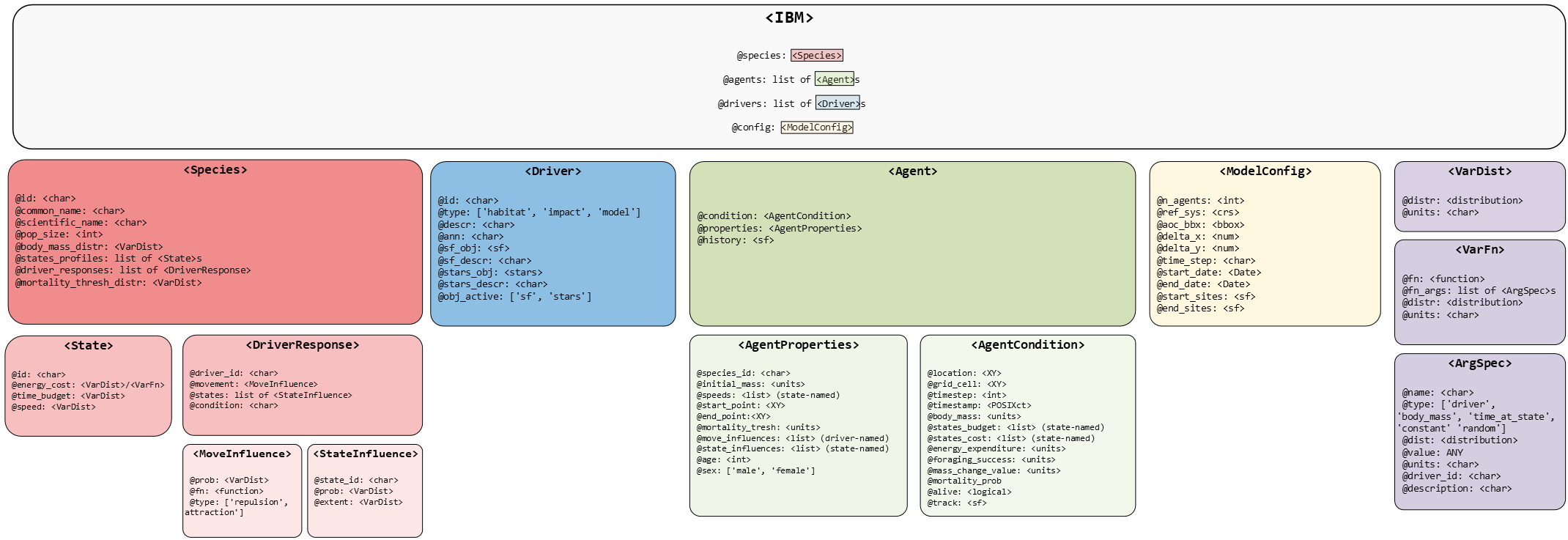
Here we use roamR to simulate the movement and energetics for a population of common guillemot (Uria aalge) on the Isle of May. For broad-scale details on the roamR package, refer to the general guide, with the general architecture repeated here:
The simulations here cover the non-breeding season (some 9 months, from July to March) under two broad scenarios:
- An environment free of Offshore Windfarms (OWFs) - nominally the status quo
- An environment with many synthetic OWF developments
The overall aim is to quantify the effects of potential displacement from these OWF developments, based on counterfactual comparisons of animal’s condition under the two scenarios. In line with the architecture of the roamR package, the simulation requires specifying the following main components:
-
IBM configuration (
[<ModelConfig>])Sundry high-level simulation controls, including the number of agents, spatial extent and geographic projection, temporal resolution, start and end dates of the model run.
-
Species-level information (
<Species>)Parameters describing the species’ biology and ecology, such as distributions for initial body mass, available activity states and associated energetic costs, movement parameters, how agents respond to environmental conditions and barriers, etc.
-
Drivers (
<Driver>)Descriptions/data that define the environment that agents may interact with or respond to e.g. population density maps, sea surface temperatures, OWF locations, coastlines, etc.
The extent to which these can be reliably populated will obviously vary across species and regions. The Isle of May Guillemot population is used here as case study due to the availability of relatively rich supporting data.
The roamR infrastructure is intentionally general and flexible, and many of its broader capabilities are not required for this example. In the following sections, we will systematically populate the relevant IBM components, before running the simulation and post-processing the results.
Settting up the IBM
We begin by defining the model settings and specifying the inputs required to initialise an IBM for this case study using roamR.
Data Availability
As a relatively well-studied species/population, many roamR components can be populated using available data. In this vignette, we draw on:
- Density maps
- SST
- Activity data
- Energetics
- Species’ bodyweight distributions
- Body mass conversion
These datasets are (a) described in detail and (b) implemented in appropriate roamR object classes in the following sections.
Note: although roamR can operate with minimal data inputs - illustrated in the alternative test case for red‑throated divers - results in such cases will be inherently more uncertain and more strongly driven by stochastic variation.
IBM configuration
The broad configuration of the IBM is specified via the function
ModelConfig(). In the interest of speed, the example
simulation here will not be large in terms of the number of agents to
run - we’ll opt for few agents (n_agents), whereas a
typical run would usually involve several thousands of individuals. For
guillemots, the non-breeding season spans roughly 9 months beginning in
early July, which we specify using the start_date and
end_date arguments. We set the temporal resolution to
one-day time steps (delta_time), meaning that agent state
updates - such as activity balancing and movement decisions - are
evaluated on a daily basis.
We’ll opt to our simulation to operate on the UTM 30N coordinate
system (ref_sys), which forms the basis for ingesting,
projecting and aligning all the spatial inputs throughout the model
workflow.
Note: the sf package is generally used for dealing with spatial data , and the interlinked stars package for spatiotemporal information.
# define UTM zone 30N
utm30 <- st_crs(32630)
Agent starting and ending locations (start_sites,
end_sites) must be supplied as <sf>
objects containing two required columns:
-
id, a unique site identifier -
prop, the proportion of agents assigned to each site.
In this example, we use the Isle of May as the sole starting
location, specified as a geometric point by its geographic
(longitude/latitude) coordinates. We do not make use of
end_sites in this simulation; agents simply remain at their
final positions once the simulation ends.
Because ModelConfig() expects spatial inputs to match
the CRS defined by ref_sys, the site must be projected to
UTM Zone 30N.
# location of colony in long/lat degrees - start/finish locations
isle_may <- st_sf(
  id = "Isle of May",
  prop = 1,
  geom = st_sfc(st_point(c(-2.5667, 56.1833))),
  crs = 4326)

# re-project to UTM 30N
isle_may <- st_transform(isle_may, crs = utm30)
In terms of bounding the simulation spatially, we’ve opted for a semi-arbitrary bounding box around the Isle of May that encompasses a large swathe of the North Sea and far to the west of the UK, which covers the bulk of the guillemot density maps. Importantly, this a hard boundary in terms of simulations - data outside this will have no influence.
# define the Area of Calculation
AoC <- st_bbox(c(xmin = 178831, ymin = 5906535,  xmax = 1174762, ymax = 6783609), crs = st_crs(utm30))
In this case study, we adopt the density-informed
movement model (movement_model, refer guidance document),
under which species-level density maps influence agent movement by
providing a spatio-temporal varying preference surface.
Passing the above configuration inputs to ModelConfig()
creates a <ModelConfig> object, which we assigned to
guill_ibm_config:
# IBM Settings - assume fixed for these simulations
guill_ibm_config <- ModelConfig(
  movement_model = "di",
  n_agents = 4,
  ref_sys = utm30,
  aoc_bbx = AoC,
  delta_time = "1 day",
  start_date = lubridate::date("2025-07-01"),
  end_date = lubridate::date("2025-07-01") + lubridate::days(9*30), # 1 month ~ 30 days
  start_sites = isle_may
)

# show created <ModelConfig> object
guill_ibm_config
#> <ModelConfig> instance with attributes:
#> • Movement Model:      Density-informed
#> • No. Agents:          4
#> • Simulation period:   2025-07-01 -- 2026-03-28 (270 days)
#> • Temporal resolution: 1 day
#> • Bounding box:        xmin: 178831  ymin: 5906535  xmax: 1174762  ymax: 6783609 [m]
#> • Projected CRS:       WGS 84 / UTM zone 30N
#> • Start site:          Simple feature with 1 feature and 2 fields [WGS 84 / UTM zone 30N]
#>               id prop                     geom
#>    1 Isle of May    1 POINT (526895.8 6226565)
#> • End site:            NA
Driver information: specifying the environment
In roamR, drivers define the environmental context with
which agents may interact with or to which they may respond. Each driver
is defined by a <Driver> object, which can be created
using the Driver() function. The scope of these will be
defined by the level of knowledge for the species of interest - at the
minimum the agents would not be responsive to the environment. Any
environmental component that can/will be functionally linked to the
animal’s behaviour (activity states or movement) or their energetic
expenditures, must be included in the definition of the environment via
the drivers.
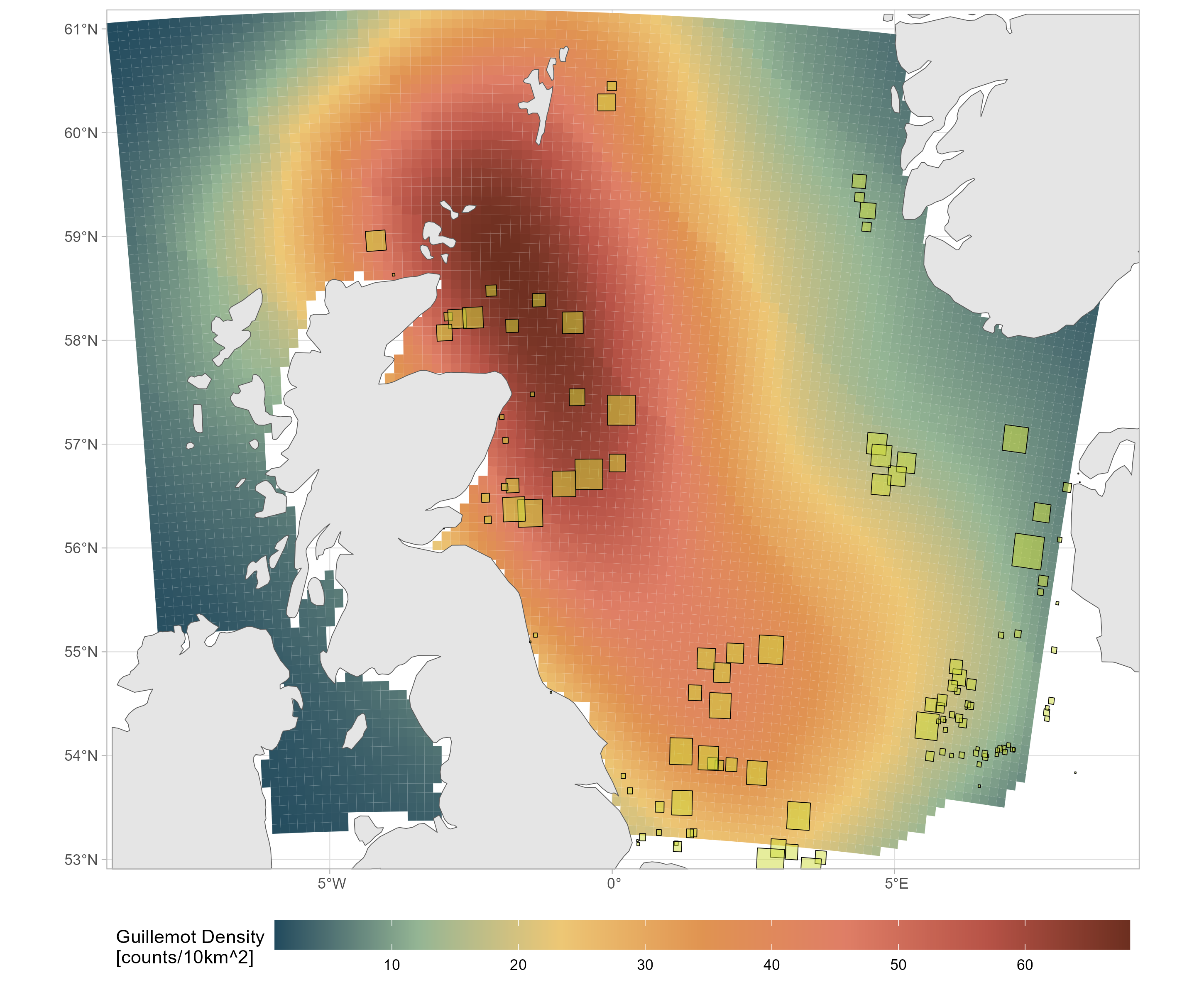
In this application to the common guillemot, the following drivers are required - all provided as spatio-temporal datacubes (2D rasters giving values for locations over time ) so the agents can query their environment at any :
Monthly species density surfaces, for both baseline and impacted scenarios (Buckingham et al. 2023). These give monthly density predictions around the UK at a 10 km^2 resolution (with bootstrap uncertainties).
Monthly energy intake maps (kJ/h), for both baseline and impacted scenarios based on density maps above, and conspecifics (other Guillemots, refer below).
Monthly average Sea Surface Temperature (SST) maps (National Oceanic and Atmospheric Administration/NOAA here).
roamR enforces a strict requirement that all input variables be accompanied by appropriate measurement units. This ensures that all computations performed during simulation are unit-aware, allowing for accurate operations and conversions.
We begin by uploading these datacubes, assigning measurement units where they are missing.
# upload available spatial surfaces

## population density maps: baseline and impacted scenarios
spec_map <- readRDS("data/bioss_spec_map.rds") |>
   mutate(density =  units::set_units(density, "counts/10km^2"))

spec_imp_map <- readRDS("data/bioss_spec_imp_map.rds") |>
   mutate(density =  units::set_units(density, "counts/10km^2"))

dpal <- hcl.colors(10, palette = "GnBu", rev = TRUE)
plot(spec_map, col = dpal, breaks = "equal")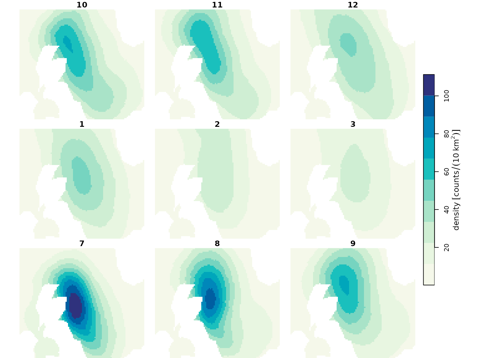
plot(spec_imp_map, col = dpal, breaks = "equal")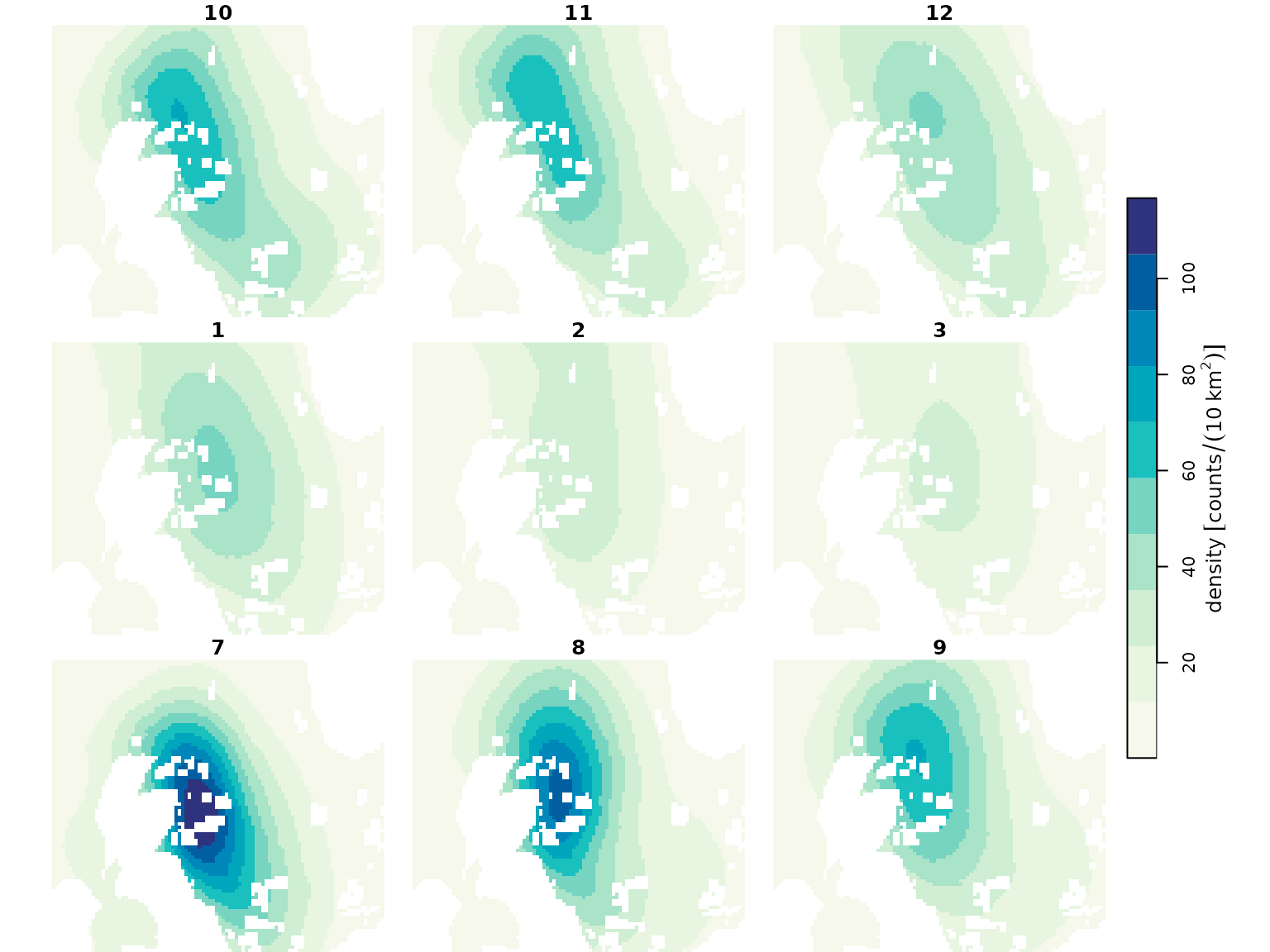
## Energy intake maps: basline and ipacted scenarios
intake_map <- readRDS("data/guill_energy_intake_map.rds")
imp_intake_map <- readRDS("data/guill_impacted_energy_intake_map.rds")

ipal <- hcl.colors(10, palette = "PurpOr", rev = TRUE)
plot(intake_map, col = ipal[length(ipal)], breaks = "equal")
plot(imp_intake_map, col = ipal, breaks = "equal")
## Sea surface temperature rasters
sst_map <- readRDS("data/sst_stars.rds")
plot(sst_map, col = hcl.colors(12, palette = "Zissou 1"), breaks = "equal")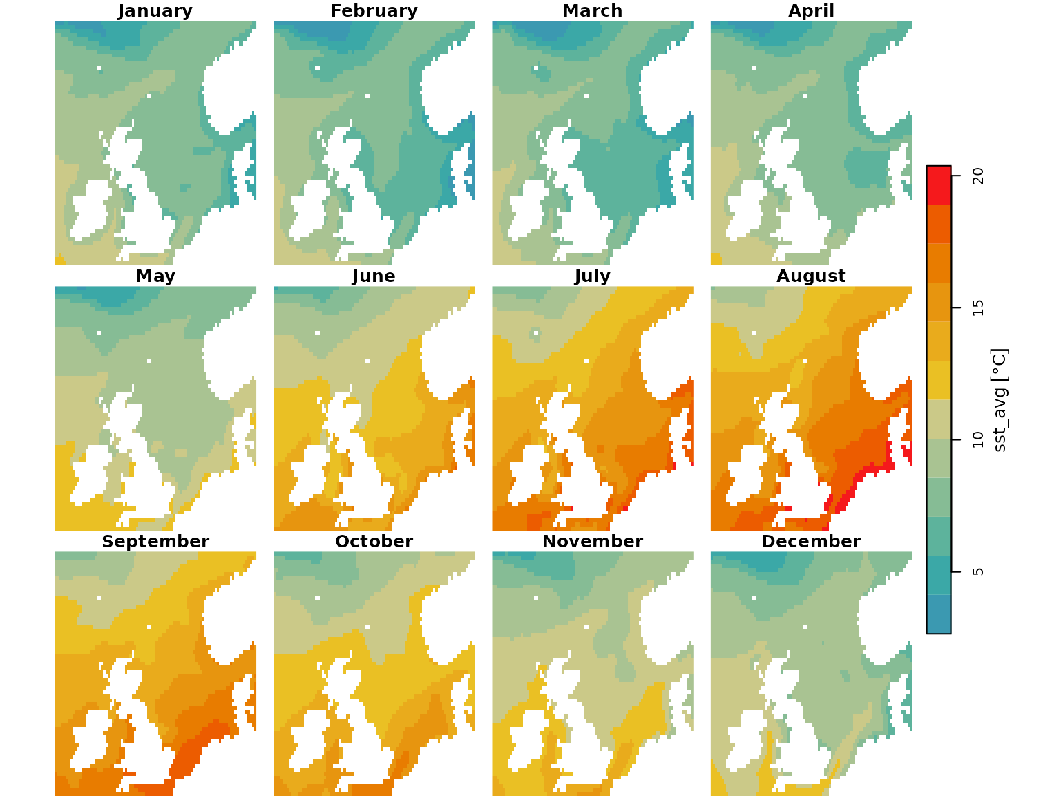
Next we specify the corresponding drivers, and stored them as a list
of <Driver> objects. Collectively these lists define
the environment the agents will move through, offering flexibility to
comprise spatial features such as coastal polygons, OWF footprints,
prey-fields, etc.
In our specific case:
Density maps are used in the density-informed movement model, guiding agents toward areas with higher habitat preference while implicitly excluding land as potential destinations. Likewise, OWF footprints are incorporated as spatial holes in the “impact” density surfaces, defining no‑go areas for OWF‑sensitive agents.
-
Energetic maps represent spatial variation in energetic gain:
in the unimpacted scenario, the energetics surface reflects an Ideal Free Distribution (IFD): on average, agents meet their energetic requirements, and their spatial distribution reflects the underlying resource landscape.
under the impacted scenario, the energetics surface incorporates displacement caused by OWFs and the resulting redistribution of conspecifics. Increased competition reduces available resources proportionally - for example, a doubling of local density leads to halved resource availability.
Sea surface temperature is used in the calculation of activity-state energetics through time, specifically affecting the energetic costs experienced by agents while on water (swimming and resting, see below).
# Set up IBM drivers

# guillemot baseline density maps
dens_drv <- Driver(
  id = "dens",
  descr = "species dens map",
  stars_obj = spec_map,
  obj_active = "stars"
)

# guillemot impacted density maps
dens_imp_drv <- Driver(
  id = "dens_imp",
  descr = "species redist map",
  stars_obj = spec_imp_map,
  obj_active = "stars"
)

# baseline energy intake maps
energy_drv <- Driver(
  id = "energy",
  descr = "energy map",
  stars_obj = intake_map,
  obj_active = "stars"
)

# impacted energy intake maps
imp_energy_drv <- Driver(
  id = "imp_energy",
  descr = "energy impact map",
  stars_obj = imp_intake_map,
  obj_active = "stars"
)

# Sea Surface Temperature
sst_drv <- Driver(
  id = "sst",
  descr = "Sea Surface Temperature",
  stars_obj = sst_map,
  obj_active = "stars"
)


# store as list, for initialisation
guill_drivers <- list(
  dens = dens_drv,
  imp_dens = dens_imp_drv,
  energy = energy_drv,
  imp_energy = imp_energy_drv,
  sst = sst_drv
)
Species information: properties underpinning individual agents
Species-level information is defined using the Species()
function, which depends on a set of input objects. For clarity and
modularity, these inputs should be prepared and specified
beforehand.
States Profile
We begin by defining the behavioural states to include in the model. Each state represents a specific activity, characterized by parameters such as energy expenditure, time allocation, and movement speed.
States are created using the State() function. roamR
supports flexible specification of state properties, allowing the
incorporation of stochastic variation at both the population and
individual (agent) level.
Here we include 4 states:
- flying
- diving
- active on water (i.e. swimming)
- inactive on water (i.e. resting)
Flying
We start with the flight state. For this simulation, we
assume the energetic cost (energy_cost) of flying for each
agent varies throughout the simulation, following a Normal distribution
with mean 507.6 kJ/h and standard deviation of 237.6 kJ/h. The source
for these figures are Elliott et al.
(2013).
Stochasticity can enter the state specification in further ways. Here
we assume that each agent has a fixed average flying speed for the
entire simulation (representing inherently faster or slower
individuals), with speeds drawn from a Uniform distribution as specified
below (speed). The proportion of time allocated to flight
at the initial time step (time_budget) is set to 0.056
h/day for all simulated agents.
# user-defined function returning a non-negative energy cost of flying
flight_cost_fn <- function(mean, sd){
  e <- rnorm(1, mean, sd)
  units::set_units((max(e, 1)), "kJ/h")
}

# define <State> object for flight activity
flight <- State(
  id = "flight",
  energy_cost = VarFn(
    flight_cost_fn,
    args_spec = list(mean = 507.6, sd = 237.6),
    units = "kJ/hour"
    ),
  time_budget = VarDist(0.056, "hours/day"),
  speed = VarDist(dist_uniform(10, 20), "m/s")
)

# inspect flight object
flight
#> An object of class "State"
#> Slot "id":
#> [1] "flight"
#>
#> Slot "energy_cost":
#> <VarFn>
#> function (mean, sd)
#> {
#>     e <- rnorm(1, mean, sd)
#>     units::set_units((max(e, 1)), "kJ/h")
#> }
#> <environment: 0x563fd872d3c0>
#>
#> Args:
#> • `mean`: 507.6
#> • `sd`: 237.6
#>
#> Output units: [kJ h-1]
#>
#> Slot "time_budget":
#> <VarDist>
#> 0.056 [h d-1]
#>
#> Slot "speed":
#> <VarDist>
#> U(10, 20) [m s-1]
To ensure biologically realistic behaviour,
flight_cost_fn() constrains sampled energy costs to a
minimum of 1 kJ/h, avoiding the occasional negative values produced by a
Normal distribution. The plots below illustrate the distributions that
will be sampled for the stochastic elements of the "flight"
state — specifically, per‑step energy costs and per‑agent flight
speeds.
## generate random samples of energy cost and flight speed
set.seed(1991)
flight_draws <- tibble(
  `Flight cost` = replicate(2000, flight_cost_fn(507.6, 237.6), simplify = FALSE) |> list_c(),
  `Flight speed` = roamR::generate(flight@speed, 2000)
)

p1 <- ggplot(flight_draws) +
  geom_density(aes(`Flight speed`), fill = "#EFEBE9", col = "gray20") +
  labs(subtitle = "Per agent at initialization")

p2 <- ggplot(flight_draws) +
  geom_density(aes(`Flight cost`), fill = "#EFEBE9", col = "gray20") +
  labs(subtitle = "Per agent at each simulation step")

(p1 + p2) + plot_annotation(title = "'flight' state: sampling distributions")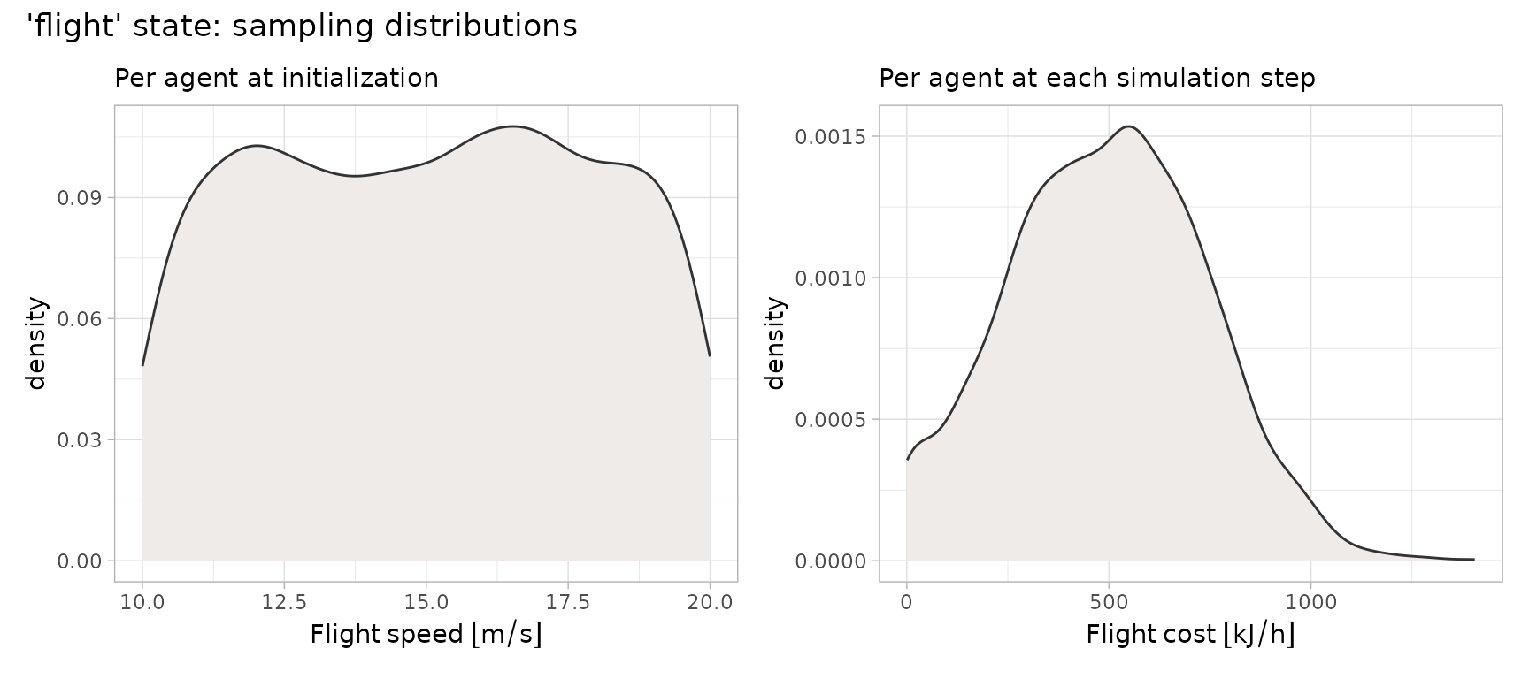
Diving
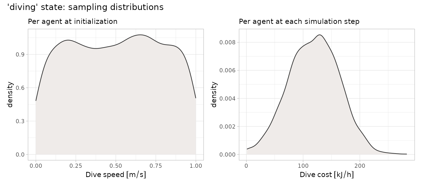
For the state representing the diving activity, the energy output is contingent on the amount of diving (Elliott et al. 2013).
Where
is the length of dive
in minutes. Here we are performing day-level calculations, meaning we
are far from simulating at the dive level, and can use a mean
dive-length without loss of generality. This is specified as parameter
t_dive in the defined diving cost function, with input
value derived from tag information.
To introduce agent‑level stochasticity, we allow the energetic
multiplier in the above equation (the leading coefficient, 3.71) to vary
among individuals. We therefore parameterise this multiplier as
alpha, assuming it follows a Normal distribution with mean
3.71 and standard deviation 1.3, such that each agent’s diving cost
fluctuates throughout the simulation. Diving energy costs are also
constrained to a minimum of 1 kJ/h.
Diving speeds are drawn from a Uniform distribution, and initial time allocated to diving is set to 3.11 h/day.
# define costing function, with non-negative cost constraint
dive_cost_fn <- function(t_dive, alpha_mean, alpha_sd){
  alpha <- rnorm(1, alpha_mean, alpha_sd)
  (max(alpha*sum(1-exp(-t_dive/1.23))/sum(t_dive)*60, 1)) |>
    units::set_units("kJ/h")
}

# Construct <State> object
dive <- State(
  id = "diving",
  energy_cost = VarFn(
    dive_cost_fn,
    args_spec = list(t_dive = 1.05, alpha_mean = 3.71, alpha_sd = 1.3),
    units = "kJ/hour"
    ),
  time_budget = VarDist(3.11, "hours/day"),
  speed = VarDist(dist_uniform(0, 1), "m/s")
)
The following plots illustrate the sampling distributions specified for drawing random values of movement speeds and energetic costs associated with diving.
Active on Water
State representing active on water (Buckingham et al. 2023) is a linear function in sea surface temperature (SST):
where the intercept has a mean of 113 and SD of 22. is a constant of 2.75.
Because this state explicitly depends on SST, we must ensure that the
corresponding driver is linked correctly within the
<State> object. This is achieved through the
args_spec argument in State(). Specifically,
we include a list element named sst, set to
"driver", which instructs roamR to retrieve SST values from
the "sst" driver defined earlier in the vignette.
The specification of the remaining attributes for this state follows the same principles used for the previous states.
# define water-active cost function, with non-negative cost constraint
active_water_cost_fn <- function(sst, int_mean, int_sd){
  int <- rnorm(1, int_mean, int_sd)
  (max(int-(2.75*sst), 1)) |>
    units::set_units("kJ/h")
}

# Construct <State> object
active <- State(
  id = "active_on_water",
  energy_cost = VarFn(
    active_water_cost_fn,
    args_spec = list(sst = "driver", int_mean = 113, int_sd = 22),
    units = "kJ/hour"
  ),
  time_budget = VarDist(10.5, "hours/day"),
  speed = VarDist(dist_uniform(0, 1), "m/s")
)
## generate random samples
set.seed(1991)

# gather cost function argument values
i_mn <- active@energy_cost@args_spec$int_mean@value
i_sd <- active@energy_cost@args_spec$int_sd@value
sst_range <- range(sst_map[[1]], na.rm = TRUE)
sst <- seq(sst_range[1], sst_range[2], by = 1)

n <- 1000

active_cost_draws <- tibble(
  sst,
  draw = list(1:n),
  `Active cost` = map(
    drop_units(sst),
    \(x) replicate(n, active_water_cost_fn(x, i_mn, i_sd), simplify = FALSE) |> list_c()
  )
) |>
  unnest(c(`Active cost`, draw))

p1 <- tibble(`Active speed` = roamR::generate(active@speed, 2000)) |>
  ggplot() +
  geom_density(aes(`Active speed`), fill = "#EFEBE9", col = "gray20") +
  labs(subtitle = "Per agent at initialization")


p2 <- active_cost_draws |>
  ggplot(aes(x = sst, y = `Active cost`)) +
  stat_lineribbon() +
  scale_fill_manual(values = c( "#EFEBE9", "#D7CCC8", "#A1887F")) +
  labs(subtitle = "Per agent at each simulation step")
  #scale_fill_brewer(palette = "Greys")

(p1 + p2) + plot_annotation(title = "'active on water' state: sampling distributions")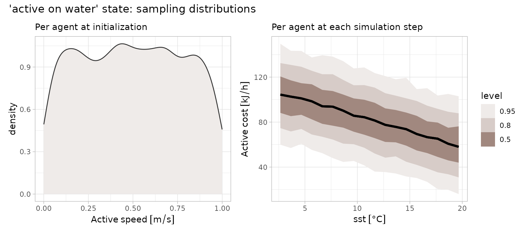
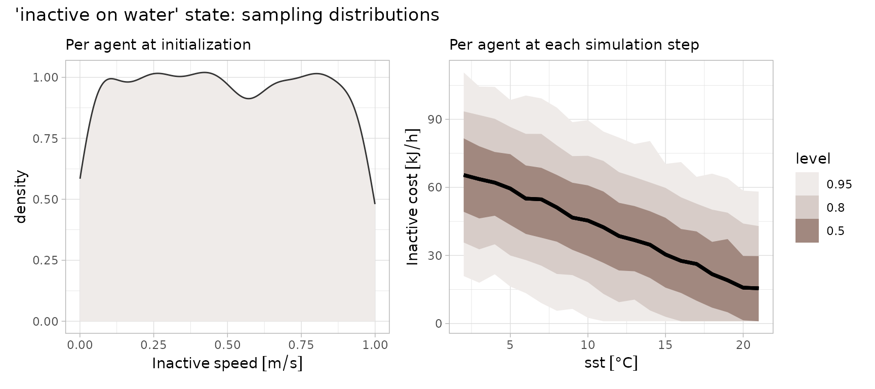
Inactive on Water
State for inactive on water (Buckingham et al. 2023), follows the same linear function in SST, but where has a mean of 72.2 and SD of 22. is similarly constant at 2.75.
inactive_water_cost_fn <- function(sst, int_mean, int_sd){
  int <- rnorm(1, int_mean, int_sd)
  (max(int-(2.75*sst), 1)) |>
    units::set_units("kJ/h")
}

inactive <- State(
  id = "inactive_on_water",
  energy_cost = VarFn(
    active_water_cost_fn,
    args_spec = list(sst = "driver", int_mean = 72.2, int_sd = 22),
    units = "kJ/hour"
  ),
  time_budget = VarDist(10.3, "hours/day"),
  speed = VarDist(dist_uniform(0, 1), "m/s")
)
Driver Responses
In this section, we define species-level, agent-specific responses to
the environmental drivers introduced and defined earlier. For the
guillemot model, we assign the density drivers - identified as
"dens" (baseline) and "dens_imp" (impacted) -
as the primary determinants of agent movement (density maps as per Buckingham et al. (2022)).
For each scenario, we also specify the probability that an agent is
influenced by the respective driver via the the prob
argument in MoveInfluence(). In the baseline case, all
agents “respond” to the density map for their movement1. In contrast, for the
"dens_imp" driver, the probability reflects how likely an
individual is to respond to the presence of an OWF installation (see
Peschko et al. (2024)). Agents that
respond to the impacted density map therefore experience altered
movement preferences, representing displacement or avoidance of OWF
footprints.
resp_dens <- DriverResponse(
  driver_id = "dens",
  movement = MoveInfluence(
    prob = VarDist(distributional::dist_degenerate(1)),
    type = "attraction",
    sim_stage = "bsln"
  )
)

resp_imp_dens <- DriverResponse(
  driver_id = "dens_imp",
  movement = MoveInfluence(
    prob = VarDist(distributional::dist_normal(0.67, sd = 0.061)),
    type = "attraction",
    sim_stage = "imp"
  )
)
Create the <Species> object
In addition to the parameters defined above, we set the remaining
species-level properties using the Species() helper
function. The body mass distribution (body_mass_distr),
used to initialise each agent’s body mass, is assumed to be Normally
distributed with parameters derived from Harris
and Wanless (1988) (with additional advice from F. Daunt,
pers. comm., 2025).
The energy-to-mass conversion rate is supplied via
energy_to_mass_distr and is treated as constant across
agents and time steps, using an estimate reported in Dunn et al. (2022).
The previously defined states and driver responses are then assembled
into lists and passed to Species() via the
states_profile and driver_responses
arguments.
guill <- Species(
  id = "guill",
  common_name = "guillemot",
  scientific_name = "Uria Aalge",
  body_mass_distr = VarDist(dist_normal(mean = 929, sd = 56), "g"),
  energy_to_mass_distr = VarDist(0.072, "g/kJ"),
  states_profile = list(
    flight,
    dive,
    active,
    inactive
  ),
  driver_responses = list(
    resp_dens,
    resp_imp_dens
  )
)
Run the IBM simulation
Now the key components of the IBM have been specified, roamR can be used for the initialisation and running of the simulations.
Initialisation
The initialisation stage performs two main tasks prior to running:
- The checking of inputs for spatial and temporal conformity, performing adjustments where needed (e.g. clipping to the AoC, required CRS transformations for consistency).
- The generation the
n_agentsas indicated in the model config object.
set.seed(1009)

guill_ibm <- xfun::cache_rds({
  rmr_initiate(
    model_config = guill_ibm_config,
    species = guill,
    drivers = guill_drivers
  )
})
#> ℹ Ensuring spatio-temporal consistency of inputs
#> ✔ Ensuring spatio-temporal consistency of inputs [77ms]
#>
#>    ℹ Driver "sst" (WGS 84 (CRS84)) transformed to match CRS specified by `model_config` (WGS 84 / UTM zone 30N).
#>    ℹ Raster of Driver "sst" warped from curvilinear to regular grid
#> ℹ Cropping spatial Drivers to AoC
#> ✔ Cropping spatial Drivers to AoC [62ms]
#>
#> ℹ Processing Activity States: "flight", "diving", "active_on_water", and "inact…
#> ✔ Processing Activity States: "flight", "diving", "active_on_water", and "inact…
#>
#> ℹ Initializing 4 Agents
#> ✔ Initializing 4 Agents [273ms]
#>
#> ℹ Set up <IBM> object
#> ✔ Set up <IBM> object [20ms]
#>
#> Model initialization done! 🚀
Running the simulation
The running of the simulation involves moving each of the initialised agents through the defined environment, with monitoring of their condition through time and determining their responses to these. Parallelisation is dealt with (and assumed to be generally used) such that individual agents are piped out to independent threads of calculation - hence the speed of a simulation is a function of the number of cores available2.
Much of the parameterisiation and data from previous sections are
encapsulated within the ibm object (guill_ibm)
passed to the simulation. Several additional parameters as per
documentation can be entered here as needed. Here we specify:
- What state(s) are feeding states or resting states - the state-balancing calculations (refer to main documentation) will increase/decrease these as required
-
feed_avg_net_energythe average net energy per unit feeding - here a tuning parameter, calculable directly as the energy required to balance the energetics equations for an average agent. -
target_energythe objective of the state rebalancing in terms of daily energy (refer to main documentation). This controls the extent agents change their feeding behaviour in response to feeding success - low success means more feeding the following day. This is expressed as a target daily net energy, which here is a modest positive value, based on empirical results of body mass at the start and end of the non-breeding season (pers. comm. F. Daunt 2025). -
smooth_body_massa use-defined function to convert energy time-series to mass. Here mass deposition occurs as a function of the preceding 7 days energy intake (pers. comm. J. Green, 2025).
plan(multisession, workers = 2)

guill_results <- xfun::cache_rds({
  run_disnbs(
    ibm = guill_ibm,
    run_scen = "baseline-and-impact",
    dens_id = "dens",
    intake_id = "energy",
    imp_dens_id = "dens_imp",
    imp_intake_id = "imp_energy",
    feed_state_id = "diving",
    roost_state_id = "inactive_on_water",
    feed_avg_net_energy = units::set_units(422, "kJ/h"),
    target_energy = units::set_units(1, "kJ"),
    smooth_body_mass = bm_smooth_opts(time_bw = "7 days"),
    waypnts_res = 1000,
    seed = 1990
  )

})
#>
#> ── Running the DisNBS Individual-Based Model ───────────────────────────────────
#> ℹ Performing validation checks on inputs and underlying data.
#> ✔ Performing validation checks on inputs and underlying data. [24ms]
#>
#> ℹ Preparing and configuring data for simulation.
#> ✔ Preparing and configuring data for simulation. [189ms]
#>
#> ℹ Simulating agents' journeys under the baseline-case scenario
#> ✔ Simulating agents' journeys under the baseline-case scenario [19.8s]
#>
#> ℹ Simulating agents' journeys under the impact-case scenario
#> ✔ Simulating agents' journeys under the impact-case scenario [17.6s]
#>
#> ✔ Model simulation finished! 🛬

plan(sequential)
Query and digest the results
roamR records an extensive amount of information from its running and monitoring of the agents. The primary output is a list, with one element for each agent. The stored agents consist of three main components (each their own class, as per the package schema):
-
properties- were drawn/set at the initialisation of the simulation from the species definition, remaining constant throughout the simulation. -
condition- the specific condition of the agent at any point in the simulation. This will be the final condition at when the simulation completes. -
history- a detailed record of elements of the agent’s condition throughout the simulation. Spatiotemporally stamped, and includes post-processed energy-to-mass conversions.
These form the basis of any downstream calculations based on the simulation outputs. When there are impact scenarios in play, there will be more than one such list, with agents paired over the impact scenarios e.g. baseline versus impact.
We can examine the agent’s simulation histories directly - here we have two scenarios, each containing a number of agents:
# two scenarios
names(guill_results)
#> [1] "agents_bsln" "agents_imp"

# several agents within each
length(guill_results$agents_bsln)
#> [1] 4

# one agents history
str(guill_results$agents_bsln[[1]]@history)
#> Classes 'sf' and 'data.frame':   272 obs. of  15 variables:
#>  $ timestep                          : int  0 1 2 3 4 5 6 7 8 9 ...
#>  $ timestamp                         : POSIXct, format: NA "2025-07-01" ...
#>  $ track_id                          : int  0 1 1 1 1 1 1 1 1 1 ...
#>  $ body_mass                         : Units: [g] num  893 859 824 875 784 ...
#>  $ body_mass_smooth                  : Units: [g] num  NA 849 850 850 850 ...
#>  $ states_budget.flight              : num  0.00234 0.00256 0.00243 0.00262 0.00228 ...
#>  $ states_budget.diving              : num  0.1298 0.0457 0.094 0.0248 0.1493 ...
#>  $ states_budget.active_on_water     : num  0.438 0.48 0.456 0.491 0.428 ...
#>  $ states_budget.inactive_on_water   : num  0.43 0.471 0.447 0.482 0.42 ...
#>  $ states_unit_cost.flight           : Units: [kJ/h] num  0 -326 -580 -268 -380 ...
#>  $ states_unit_cost.diving           : Units: [kJ/h] num  0 -176.8 -210.4 -138.4 -87.9 ...
#>  $ states_unit_cost.active_on_water  : Units: [kJ/h] num  0 -97.5 -91.3 -67 -109.7 ...
#>  $ states_unit_cost.inactive_on_water: Units: [kJ/h] num  0 -54.2 -20.1 -38.5 -40.2 ...
#>  $ energy_expenditure                : Units: [kJ] num  0 -462 -951 -250 -1511 ...
#>  $ geometry                          :sfc_POINT of length 272; first list element:  'XY' num  526896 6226565
#>  - attr(*, "sf_column")= chr "geometry"
#>  - attr(*, "agr")= Factor w/ 3 levels "constant","aggregate",..: NA NA NA NA NA NA NA NA NA NA ...
#>   ..- attr(*, "names")= chr [1:14] "timestep" "timestamp" "track_id" "body_mass" ...
Comparing scenarios
Here we extract the history from agents under the two scenarios for
comparison. All agents over both scenarios are combined into one dataset
- guill_history.
#> Simple feature collection with 2176 features and 19 fields
#> Geometry type: POINT
#> Dimension:     XY
#> Bounding box:  xmin: 363772.8 ymin: 5958868 xmax: 1143527 ymax: 6741622
#> Projected CRS: WGS 84 / UTM zone 30N
#> First 10 features:
#>    scenario agent timestep  timestamp track_id    body_mass body_mass_smooth
#> 1  baseline     1        0       <NA>        0 892.7471 [g]           NA [g]
#> 2  baseline     1        1 2025-07-01        1 859.4652 [g]     849.4795 [g]
#> 3  baseline     1        2 2025-07-02        1 824.2810 [g]     849.7302 [g]
#> 4  baseline     1        3 2025-07-03        1 874.7630 [g]     849.9787 [g]
#> 5  baseline     1        4 2025-07-04        1 783.9642 [g]     850.2197 [g]
#> 6  baseline     1        5 2025-07-05        1 915.4553 [g]     850.4383 [g]
#> 7  baseline     1        6 2025-07-06        1 867.7901 [g]     850.6294 [g]
#> 8  baseline     1        7 2025-07-07        1 792.0637 [g]     850.7875 [g]
#> 9  baseline     1        8 2025-07-08        1 880.2132 [g]     850.9198 [g]
#> 10 baseline     1        9 2025-07-09        1 836.0787 [g]     851.0286 [g]
#>    states_budget.flight states_budget.diving states_budget.active_on_water
#> 1           0.002336644           0.12976717                     0.4381207
#> 2           0.002562265           0.04573934                     0.4804247
#> 3           0.002432712           0.09398871                     0.4561334
#> 4           0.002618594           0.02476087                     0.4909863
#> 5           0.002284259           0.14927654                     0.4282986
#> 6           0.002685079           0.00000000                     0.5034522
#> 7           0.002592919           0.03432306                     0.4861722
#> 8           0.002314083           0.13816943                     0.4338905
#> 9           0.002638662           0.01728688                     0.4947491
#> 10          0.002476153           0.07781004                     0.4642786
#>    states_budget.inactive_on_water states_unit_cost.flight
#> 1                        0.4297755           0.0000 [kJ/h]
#> 2                        0.4712737        -326.0301 [kJ/h]
#> 3                        0.4474452        -580.4143 [kJ/h]
#> 4                        0.4816342        -267.6850 [kJ/h]
#> 5                        0.4201406        -380.0569 [kJ/h]
#> 6                        0.4938627        -540.9809 [kJ/h]
#> 7                        0.4769118        -458.9594 [kJ/h]
#> 8                        0.4256260        -452.3054 [kJ/h]
#> 9                        0.4853253        -173.1052 [kJ/h]
#> 10                       0.4554352        -818.3772 [kJ/h]
#>    states_unit_cost.diving states_unit_cost.active_on_water
#> 1           0.00000 [kJ/h]                   0.00000 [kJ/h]
#> 2        -176.78357 [kJ/h]                 -97.52233 [kJ/h]
#> 3        -210.44304 [kJ/h]                 -91.34800 [kJ/h]
#> 4        -138.40550 [kJ/h]                 -66.99671 [kJ/h]
#> 5         -87.91532 [kJ/h]                -109.67183 [kJ/h]
#> 6         -90.63622 [kJ/h]                -123.11517 [kJ/h]
#> 7         -87.63698 [kJ/h]                 -24.80227 [kJ/h]
#> 8         -66.87361 [kJ/h]                -114.61540 [kJ/h]
#> 9        -178.81558 [kJ/h]                 -82.01091 [kJ/h]
#> 10       -142.40802 [kJ/h]                 -74.93577 [kJ/h]
#>    states_unit_cost.inactive_on_water energy_expenditure       Date month
#> 1                     0.000000 [kJ/h]        0.0000 [kJ]       <NA>    NA
#> 2                   -54.202340 [kJ/h]     -462.2480 [kJ] 2025-07-01     7
#> 3                   -20.072190 [kJ/h]     -950.9176 [kJ] 2025-07-02     7
#> 4                   -38.494312 [kJ/h]     -249.7781 [kJ] 2025-07-03     7
#> 5                   -40.235387 [kJ/h]    -1510.8728 [kJ] 2025-07-04     7
#> 6                    -1.000000 [kJ/h]      315.3926 [kJ] 2025-07-05     7
#> 7                    -1.465116 [kJ/h]     -346.6240 [kJ] 2025-07-06     7
#> 8                   -37.139635 [kJ/h]    -1398.3800 [kJ] 2025-07-07     7
#> 9                   -50.721084 [kJ/h]     -174.0815 [kJ] 2025-07-08     7
#> 10                   -1.000000 [kJ/h]     -787.0601 [kJ] 2025-07-09     7
#>    suscep                 geometry
#> 1   FALSE POINT (526895.8 6226565)
#> 2   FALSE POINT (543716.2 6248777)
#> 3   FALSE POINT (543716.2 6248777)
#> 4   FALSE POINT (543716.2 6248777)
#> 5   FALSE POINT (543716.2 6248777)
#> 6   FALSE POINT (543716.2 6248777)
#> 7   FALSE POINT (543716.2 6248777)
#> 8   FALSE POINT (543716.2 6248777)
#> 9   FALSE POINT (543716.2 6248777)
#> 10  FALSE POINT (543716.2 6248777)
Body mass traces
We can examine a small number of agents graphically - here their body mass histories as implied by the simulated energetics. Note roamR at its heart simulates energetics, so conversion functions from energy to mass are specified by the user. Here the primary conversion figure is from Dunn et al. (2022), relating energy to grams of body mass.
p_bdm <- guill_history |>
  ggplot() +
  geom_line(aes(x = Date, y = body_mass_smooth, col = scenario), linewidth = 1) +
  scale_colour_manual(values = c("#191970", "#E53935"), name = "Scenario") +
  theme(legend.position = "bottom") +
  facet_wrap(~agent, ncol = 2, scales = "free")

p_bdm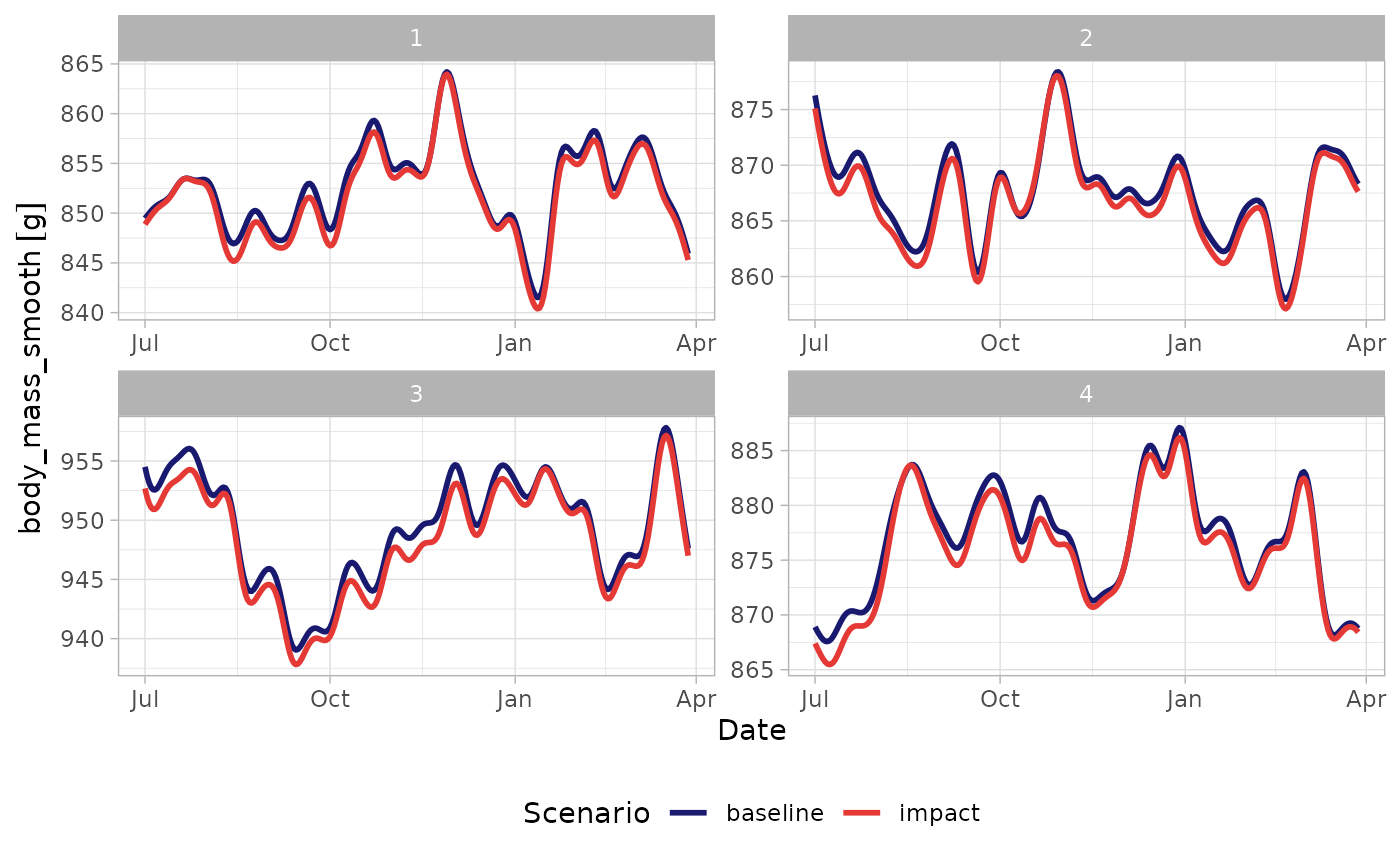
Agent tracks
Similarly movement tracks for select agents over time can be visualised, under the two impact scenarios. Here we separate by a property of the agent - those that were assigned susceptibility to OWF in the agent initialisation - recalling this was a stochastic specification at the species level.
p_tracks <- guill_history |>
  drop_na(timestamp) |>
  filter(suscep == FALSE) |>
  filter(agent == last(agent)) |>
  ggplot() +
  stars::geom_stars(data = spec_imp_map) +
  geom_sf(aes(col = scenario), size = 2) +
  scale_colour_manual(values = c("#191970", "#E53935"), name = "Scenario") +
  scale_fill_fermenter(
    guide = "colourbar",
    palette = "GnBu",
    na.value = "white",
    direction = 1,
    n.breaks = 8,
    name = "Density\n[counts/10km^2]"
  ) +
  facet_wrap(~month, ncol = 3) +
  labs(
    title = "Monthly movement tracks for a non-sensitive agent",
    subtitle = "Baseline Vs Impacted scenarios"
  ) +
  theme(legend.position = "bottom")

p_tracks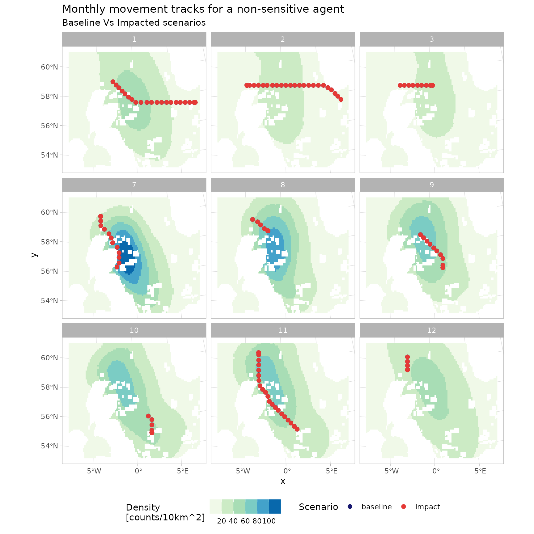
p_tracks <- guill_history |>
  drop_na(timestamp) |>
  filter(suscep == TRUE) |>
  filter(agent == last(agent)) |>
  ggplot() +
  stars::geom_stars(data = spec_imp_map) +
  geom_sf(aes(col = scenario), size = 2) +
  scale_colour_manual(values = c("#191970", "#E53935"), name = "Scenario") +
  scale_fill_fermenter(
    guide = "colourbar",
    palette = "GnBu",
    na.value = "white",
    direction = 1,
    n.breaks = 8,
    name = "Density\n[counts/10km^2]"
  ) +
  facet_wrap(~month, ncol = 3) +
  labs(
    title = "Monthly movement tracks for a sensitive agent",
    subtitle = "Baseline Vs Impacted scenarios"
  ) +
  theme(legend.position = "bottom")

p_tracks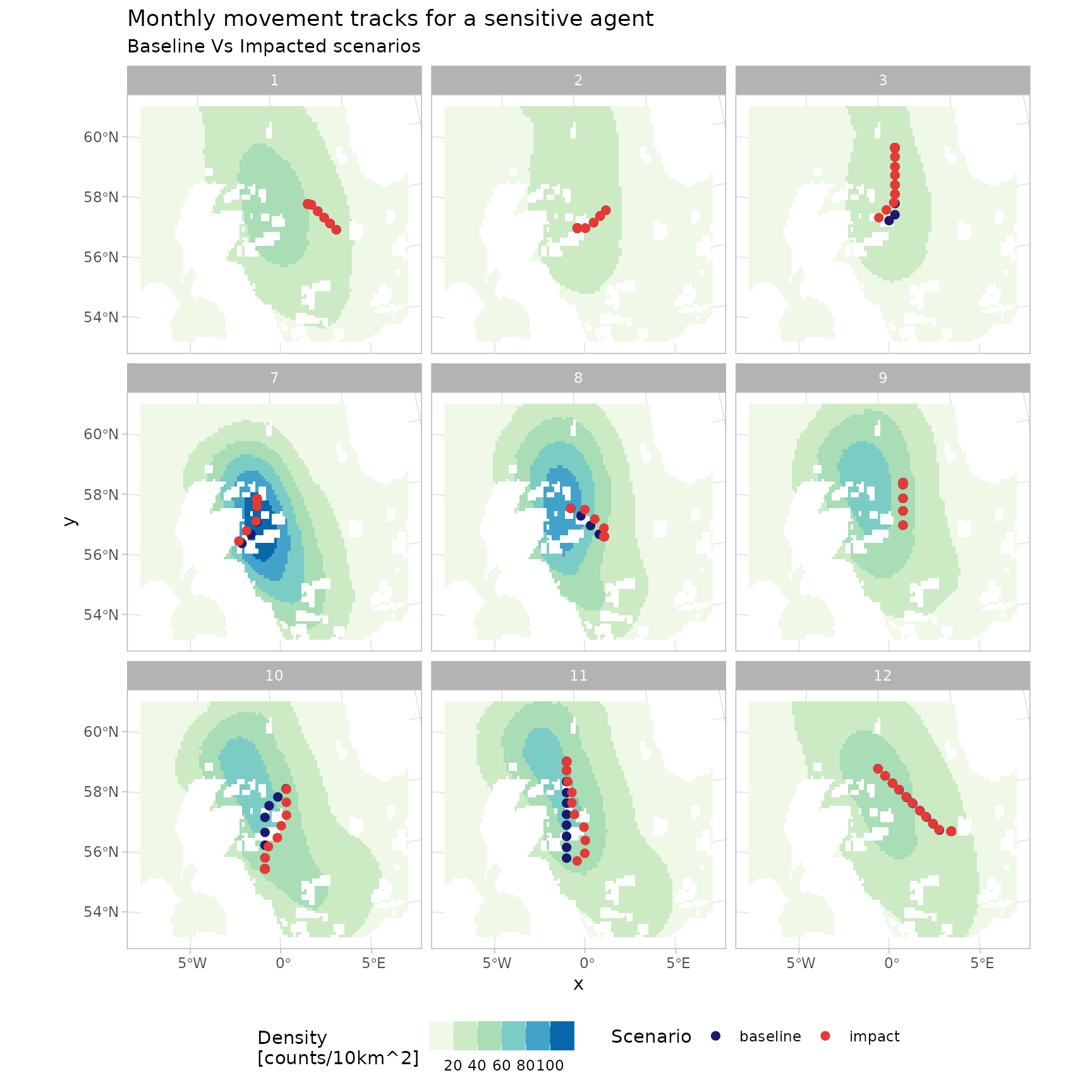
The figure below shows the movement of 250 agents over the full duration of a simulation, for the same model configuration but with a larger number of simulated agents. The animation depicts how agents’ movement patterns are informed by the monthly density surfaces under the impacted scenario, while also highlighting how individuals respond to the OWF footprints as tolerated passage zones according to their assigned susceptibility.
# Creating animation of movements for a sample of the simulation agents, under
# the impact scenario

# create copy of impacted density map, with March layer replicated as additional
# April layer for animation rendering purposes
dens_imp <- spec_imp_map
dens_imp_apr <- filter(dens_imp, month == 3) |>
  st_set_dimensions("month", values = 4)
dens_imp <- c(dens_imp, dens_imp_apr, along = "month")

# convert numeric months to Date, for consistency with history outputs
month_num <- st_get_dimension_values(dens_imp, "month")
dens_imp <- st_set_dimensions(
  dens_imp,
  which = "month",
  values = as.Date(sprintf("202%i-%i-01", ifelse(month_num <= 4, 6, 5), month_num)),
  names =  "Date"
)

# generate animation
anim <- guill_history_long |>
  drop_na(timestamp) |>
  filter(
    scenario == "impact",
    agent %in% unique(agent)[1:250]
  ) |>
  mutate(
    owf_sensitive = fct_rev(
      ifelse(owf_sensitive, "OWF Sensitive", "OWF Non-sensitive")
    )
  ) |>
  ggplot() +
  stars::geom_stars(data = dens_imp) +
  geom_sf(aes(col = owf_sensitive), size = 1.6, alpha = 0.3) +
  coord_sf(expand = FALSE) +
  scale_fill_fermenter(
    guide = "colourbar",
    palette = "GnBu",
    na.value = "white",
    direction = 1,
    n.breaks = 8,
    name = "Density\n[counts/10km^2]"
  ) +
  scale_colour_manual(
    #values = c("#E53935", "#424242"),
    values = c("#EF6C00", "#6A1B9A"),
    guide = guide_legend(position = "bottom", title = NULL)
  ) +
  transition_time(Date) +
  labs(
    title = "Impact Scenario",
    subtitle = "Date: {frame_time}",
    x = NULL, y = NULL
  )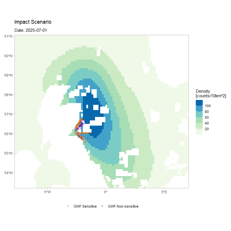
Use of counterfactals
Quantification of the impact of the perturbation can be done on any of the defined agent condition (and/or history), but for consenting the utility is through EIAs that likely use:
- Cumulative net energy
- Season-end body mass or mass change
- Distributions of activity/behavioural states
- Minimum body mass over the season
- Mortality
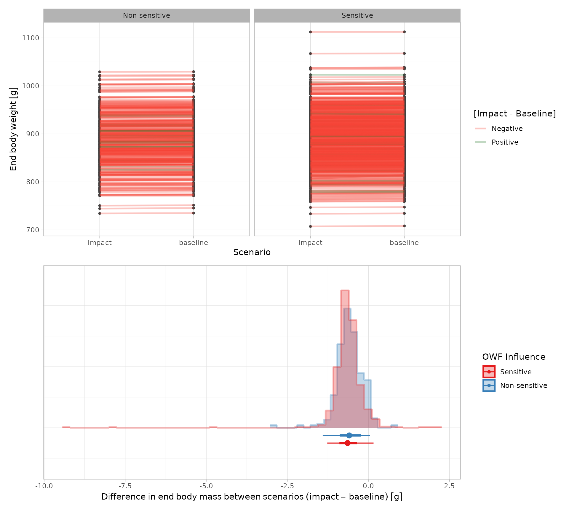
These are not single values, but distributions representing the variability in the simulated populations. For example, the plots in the next figure compare the distribution of end‑of‑simulation body masses between paired baseline and impact runs, from an model re-run with 1000 agents. Most agents show reduced final body weights under the impacted scenario, with the magnitude of this reduction slightly greater in OWF‑susceptible individuals.
While being directly informative at a population level (e.g. the mean %-age of the population lost), the output distributions are tangible for down-stream calculations. The most obvious application being in Population Viability Analyses (PVAs) that are frequently required in EIAs for consenting. There the counterfactuals may use:
- Increases in mortality/proportional reductions in population size
- Relationships between body mass and reproductive success, to alter PVA demographic parameters
For example, Natural England provide an R PVA toolset here nepva, frequently used in consenting, where the distributions of productivity can be specified under differing scenarios. The PVAs provide monte-carlo simulations of projected population sizes, which are matched (impact-to-baseline) to give population-level counterfactuals of impacts. The DisNBS simulations can be used to estimate these productivities.