4  Example Krill MSE

Showcasing the application of a Management Strategy Evaluation to the Krill fishery using the openMSE tool

4.1 Introduction

4.2 Set-up MSE

4.2.1 Build the base-case Operating Model

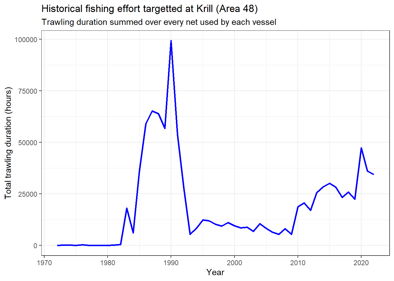
Compute time-series of yearly total fishing effort targeted at Krill in terms of trawling duration in hours (summed over each net in each vessel) in the whole Statistical Area 48 (source: CCAMLR Secretariat 2023).

# filter effort for krill in all subareas of 48
effort_krill_48 <- effort_ccamlr |> 
  filter(
    target_species_code == "KRI",
    asd_code %in% as.character(c(48, 481:486))
    )

yearly_trawl_hrs_krill_48 <- effort_krill_48 |> 
  group_by(year) |> 
  summarise(trawl_hrs = sum(trawl_duration_hours, na.rm = TRUE))

ggplot(yearly_trawl_hrs_krill_48) +
  geom_line(aes(x = year, y = trawl_hrs), col = "blue", linewidth = 1) +
  labs(
    x = "Year", 
    y = "Total trawling duration (hours)", 
    title = "Historical fishing effort targetted at Krill (Area 48)",
    subtitle = "Trawling duration summed over every net used by each vessel"
  )

The base-case OM is specified next, taking the PR estimates and maturity ogive defined under scenario scn-2 of the openMSE-Grym approximation analysis presented in Part 1 of this project (Table 2.3). This scenario comprises random draws of natural mortality rate \(M\) that are closest to the range of estimates presented in Pakhomov (1995), and maturity ogive estimates recommended in Maschette et al. (2021).

[Add main differences to OMs specified in openMSE-Gryn approximation]

# Selecting scenario "scn-2"
krill_pars <- grym_setups |> 
  filter(scenario_id == "scn-2")
  
krill_base_OM <- build_krill_OM(
  om_name = "krill_base_case", 
  maxage = last(unlist(krill_pars$Ages)), 
  nyears = nrow(yearly_trawl_hrs_krill_48), 
  LenCV = c(0.05,   0.08),                     # low variation in length-at-age
  effort = yearly_trawl_hrs_krill_48$trawl_hrs,
  qinc = c(0.0),                             # no increase in fishing efficiency
  M_draws = krill_pars$prRecruitPars$`PR-emm21`$M, 
  RCV_draws = krill_pars$prRecruitPars$`PR-emm21`$CV, 
  n_iter = krill_pars$n_iter, 
  proj_yrs = krill_pars$n.years, 
  maxF = krill_pars$Fmax, 
  seed = 101
)

write_rds(krill_base_OM, "inputs/krill_base_OM.rds")

Next we render the OM report documenting all the parameter values specified under the base-case OM, along with the rationale behind their selection. The base-case OM report is available in Appendix B.

# Modified versions of the MSEtool scripts solve bugs, in addition to adding the
# inclusion and  better integration in another document as an embedded html
source("../MSEtool_fixes/OM_init_doc_dmp.R")
source("../MSEtool_fixes/OM_plots_dmp.R")

OMdoc(
  OM = krill_base_OM,
  openFile = FALSE,
  rmd.source = "OM_krill_mse_base.rmd",
  bib_file = "../references.json",
  html_theme = "lumen", 
  inc_title = FALSE
)

4.2.2 Specify Management Procedures

[FO->] The choice of MPs applicable to the krill stock is conditioned by their data requirements. The krill fishery can be classified as data-limited, with mostly time-series of catches and effort available on a consistent basis. There are frequent scientific surveys but only cover specific sub-areas of the management region [<-FO]

The following assumptions are required in terms of data availability in order to apply the MPs described in Table 4.1:

• Time-series of catch at length can be estimated using length-frequency data collected from observer sampling.

• Time-series of fishery-dependent CPUE are obtainable from annual catch and effort data. These CPUE estimates can be standardized to provide a suitable relative index of abundance.

• Prescribed MSY-based reference points can be either calculated (e.g. the method by Martell and Froese, 2012) or specified via expert elicitation.

Code

MPs <- read_xlsx(
  "krill applicable MPs.xlsx", 
  sheet = "picked_MPs_description"
) 

MPs_names <- MPs$Name

MPs |> 
  flextable() |> 
  add_header_row(
    values = c("General Category", "Name", "Description", "Data Requirements"), 
    colwidths = c(1, 1, 1, 5)
  ) |> 
  merge_v( j = 1:3, part = "header") |>
  merge_v( j = 1, part = "body") |> 
  align(i = 1:2, align = "center", part = "header") |>
  align(j = 4:8, align = "center", part = "body") |> 
  footnote(
    #i = ~select(Name, starts_with("Fdem")), j = 8, 
    i = ~str_detect(Name, "Fdem"), 
    j = "Prescribed F_MSY/M",
    value = as_paragraph(
    "Requirement according to documentation and input validation in source code. However FMSY_M is not used anywhere in `Fdem_` functions... so assuming requirement is non-valid."
    ), 
    ref_symbols = "ǂ") |> 
  bg(j = ~`Catch series`, i = ~str_detect(`Catch series`, "X"), bg = "#E1F5FE", part = "body") |> 
  bg(j = ~`Index series`, i = ~str_detect(`Index series`, "X"), bg = "#E1F5FE", part = "body") |> 
  bg(j = ~`Catch@length series`, i = ~str_detect(`Catch@length series`, "X"), bg = "#E1F5FE", part = "body") |>  
  bg(j = ~`Life history parameters`, i = ~str_detect(`Life history parameters`, "X"), bg = "#E1F5FE", part = "body") |> 
  bg(j = ~`Prescribed F_MSY/M`, i = ~str_detect(`Prescribed F_MSY/M`, "X"), bg = "#E1F5FE", part = "body") |> 
  bg(bg = "#FFFFFF", part = "header") |>
  set_table_properties(
    layout = "autofit",
    opts_word = list(split = TRUE),
    opts_html = list(scroll = list(height = "800px"))
  ) 

Table 4.1: Management Plans (MPs) selected for the MSE application to the krill fishery

General Category	Name	Description	Data Requirements
			Catch series	Index series	Catch@length series	Life history parameters	Prescribed F_MSY/M
Status-quo	AvC	Constant TAC over projection period based on average historical catch. Represents the "status quo" management option.	X
Stabilisation	Islope1	TAC ajusted incrementally to maintain stable CPUE or abundance index. Based on average recent catch (last 5 years) and the trajectory of index of abundance over the past 5 years.	X	X
	Islope4	Similar to Islope1, but more precautionary. Uses a fraction (0.6) of average recent catch and forces slower changes in TAC in response to changes in cpue/index trajectory	X	X
	LstepCC1	TAC adjusted stepwise in relation to recent changes in mean length of recent catches. Takes the average historical catch (last 5 years) and applies a (upwards or downwards) step change depending on the ratio between mean length in recent catch (passt 5 years) and mean length in historical catches (last 10 years).	X		X
	LstepCC4	Similar toLstepCC1 but more precautionary. Uses a fraction (0.7) of average historical catch	X		X
Target-based	Itarget1	TAC adjusted to achieve a target CPUE/index. Based on average historical catch (last 5 years) and adjustment term expressing deviations between historical, recent and target indices. Target index defined as 1.5 of average index over the last 10 years of historical period. Recent average index calculated from past 5 years.	X	X
	Itarget4	Similar to Itarget1 but more precautionary. Uses a fraction (0.7) of average historical catch and target index is higher (2.5 of average historical index)	X	X
	Ltarget1	TAC incrementally adjusted to reach a target mean length in catches. Based on average historical catch (last 5 years) and adjustment term expressing deviations between historical, recent and target mean lengths. Target mean length defined as 1.05 of average length over the last 10 years of historical period. Recent average length in catch calculated from past 5 years	X		X
	Ltarget4	Similar to Ltarget1 but more precautionary. Uses a fraction (0.8) of average historical catch and target mean length is higher (1.15 of historical mean length)	X		X
	L95target	Same as Ltarget1 but here the target mean length is based on the length at maturity rather than an arbitrary multiplicative	X		X	X
	L95target4	As L95target but more precautionary. Uses a fraction (0.8) of average historical catch	X		X	X
MSY-based	Fdem_ML	Annual TAC set for harvesting at MSY levels based on F_MSY. F_MSY calculated as r/2, where r Is the intrinsic rate of population growth. r is estimated from life history parameters. Current abundance estimated from mean length	X		X	X	Xǂ
	Fdem_ML_25	As Fdem_ML but with a precautionary buffer of 0.25 of the recommended TAC	X		X	X	Xǂ
	Fdem_ML_50	As Fdem_ML but with a precautionary buffer of 0.50 of the recommended TAC	X		X	X	Xǂ
	Fdem_ML_75	As Fdem_ML but with a precautionary buffer of 0.75 of the recommended TAC	X		X	X	Xǂ
	SPMSY	Sets TAC to achieve harvesting at MSY. MSY estimated from Martell and Froese surplus production model. Stock trajectories estimated based on trends in catch data and life-history information	X			X
	SPMSY_25	As SPMSY but with a precautionary buffer of 0.25 of the recommended TAC	X			X
	SPMSY_50	As SPMSY but with a precautionary buffer of 0.50 of the recommended TAC	X			X
	SPMSY_75	As SPMSY but with a precautionary buffer of 0.75 of the recommended TAC	X			X
	DD	Sets TAC to achieve exploitation at UMSY, i.e. the harvest rate (the fraction of population being harvested every year) that will produce MSY. UMSY estimated from a simple delay-difference model (described in chap 9 of Hilborn and Walters, 1992) using time-series of catch and index of abundance	X	X		X
	DD_25	As DD but with a precautionary buffer of 0.25 of the recommended TAC	X	X		X
	DD_50	As DD but with a precautionary buffer of 0.50 of the recommended TAC	X	X		X
	DD_75	As DD but with a precautionary buffer of 0.75 of the recommended TAC	X	X		X
	DD4010	Similar to DD but superimposing a 40-10 HCR to constrain TAC recommendation as a function of depletion (B/B0). 40-10 rule specifies that the stock is not fished if depletion < 10% (i.e. TAC = 0), while TAC is set at UMSY levels (as DD) if depletion > 40%. If depletion is between 10 and 40%, TAC follows a linear increase from 0 to 100% UMSY levels.	X	X		X
	DD4010_25	As DD4010 but with a precautionary buffer of 0.25 of the recommended TAC	X	X		X
	DD4010_50	As DD4010 but with a precautionary buffer of 0.50 of the recommended TAC	X	X		X
	DD4010_75	As DD4010 but with a precautionary buffer of 0.75 of the recommended TAC	X	X		X
Yield-per-recruit	BK_ML	Annual TAC based on F_Max. F_max derived using length at first capture relative to L_inf and vB growth parameter K. Current vulnerable abundance estimated from recent catches and F, with F estimated from mean length	X		X	X
	BK_ML_25	As BK_ML but with a precautionary buffer of 0.25 of the recommended TAC	X		X	X
	BK_ML_50	As BK_ML but with a precautionary buffer of 0.50 of the recommended TAC	X		X	X
	BK_ML_75	As BK_ML but with a precautionary buffer of 0.75 of the recommended TAC	X		X	X
	YPR_ML	TAC set to achieve harvest at F_0.1. Yield-per-recruit curve calculated from an age-structured model at equilibrium with life-history and selectivity parameters sampled from OM. Current abundance inferred from an estimate of Z calculated from mean length in catches and life-history parameters	X		X	X
ǂRequirement according to documentation and input validation in source code. However FMSY_M is not used anywhere in `Fdem_` functions... so assuming requirement is non-valid.

4.2.3 Set Performance Metrics

[Add details on newly introduced performance metrics]

Code

esc_metric <- ESC(short_krill_mse)
pd_metric <- PD(short_krill_mse)
ssb_fvu_metric <- SSB_FvU(short_krill_mse, Ref = 0.70)
yrc_metric <- YRC(short_krill_mse)
lty_metric <- LTY(short_krill_mse)
aavy_metric <- AAVY(short_krill_mse)

PMs <- tribble(
  ~ Category,         ~ Name,     ~ Description,       ~ Detail, 
  "Spawning Biomass",  "ESC",     esc_metric@Name,      esc_metric@Caption,
  "Spawning Biomass",  "PD",      pd_metric@Name,       pd_metric@Caption,
  "Spawning Biomass",  "SSB_FvU", ssb_fvu_metric@Name,  ssb_fvu_metric@Caption,
  "Yield",             "YRC",     yrc_metric@Name,      yrc_metric@Caption,
  "Yield",             "LTY",     lty_metric@Name,      lty_metric@Caption,
  "Yield",             "AAVY",    aavy_metric@Name,     aavy_metric@Caption
)


PMs |> 
  flextable() |> 
  merge_v(j = ~Category) |> 
  fix_border_issues()  |> 
  footnote(
    i = ~ str_detect(Name, "ESC|PD"),
    j = "Name",
    value = as_paragraph("CCAMLR's default metrics"), ref_symbols = "ǂ")

Table 4.2: Performance metrics (PMs) used for the MSE of the krill fishery. Metrics SSB_FvU and YRC are averaged across simulations

Category	Name	Description	Detail
Spawning Biomass	ESCǂ	Escapement: Final Spawning Biomass relative to Virgin Spawning Biomass	median(SSB at Year 20)/median(SSB0)
	PDǂ	Depletion: Projected Spawning Biomass relative to Virgin Spawning Biomass	Prob. min(SSB) < 0.2 SSB0 (Years 1 - 20)
	SSB_FvU	Proportion of projection years with precautionary levels of exploitation	Proportion of years with SSB > 0.7 Unfished SSB (Years 1-20)
Yield	YRC	Projected Average Yield relative to Historical Average Yield	Prob. Average Projected Yield (Years 11-20) > Average Historical Yield (-9-0)
	LTY	Average Yield relative to Reference Yield (Years 11-20)	Prob. Yield > 0.5 Ref. Yield (Years 11-20)
	AAVY	Average Annual Variability in Yield (Years 1-20)	Prob. AAVY < 20% (Years 1-20)
ǂCCAMLR's default metrics

4.2.4 Generate Operating models for robustness testing

Considering five cases for testing the robustness of results under the base-case MSE (Table 4.3):

1. Sensitivity to higher variability in length-at-age (parameter LenCV)

2. Increase in catchability for the projection period (parameter qinc), i.e. fishing becomes more efficient and one unit of effort will lead to higher fishing mortality. Setting it to 1% annual increase (resulting in a 20% increase in fishing efficiency after a 20 year projection), to express advances in e.g. gear technology, generalized use of continuous fishing systems, etc.

3. Presence of persistent bias in reported catches (parameter Cbiascv), e.g. due to inconsistencies in the estimation of green weight. A CV of 5% implies that 95% of simulations are between 90% and 110% of the true simulated catches.

4. Presence of hyperstability in the estimation of abundance (parameter beta), i.e. acknowledging that estimated CPUE indices may decrease slower than the true actual abundance. This phenomenon may occur, for instance, if fishing vessels tend to move uni-directionally across sub-areas during each fishing season while krill spatial distribution is uniform.

5. Presence of persistent bias in estimates of natural mortality rate (parameter Mbiascv), e.g. as a by-product of the Proportional Recruitment method. A CV of 5% implies that 95% of simulations are between 90% and 110% of the true simulated natural mortality.

Code

rbstn_vals <- list(
  LenCV = c(0.15, 0.20),
  qinc = c(0.01, 0.01),
  Cbiascv =  0.05,
  beta = c(0.8, 0.9),
  Mbiascv = 0.05
)

rbstn_tbl <- tribble(
  ~"Robustness Test ID", ~"OM Parameter",    ~"Base-case",                            ~"Robustness",
        "Length@Age",         "LenCV",  "[0.05, 0.08]",    glue("[{toString(rbstn_vals$LenCV)}]"),
   "Fishing-efficiency",          "qinc",        "[0, 0]",     glue("[{toString(rbstn_vals$qinc)}]"),
           "Catch-bias",       "Cbiascv",             "0",    glue("{toString(rbstn_vals$Cbiascv)}"),
       "Hyperstability",          "beta",        "[0, 0]",     glue("[{toString(rbstn_vals$beta)}]"),
               "M-bias",       "Mbiascv",             "0",    glue("{toString(rbstn_vals$Mbiascv)}"),
  ) 

flextable(rbstn_tbl) |> 
  set_table_properties(width = 0.75, layout = "autofit")

Table 4.3: Parameter values used in robustnes tests applied to the krill base-case MSE

Robustness Test ID	OM Parameter	Base-case	Robustness
Length@Age	LenCV	[0.05, 0.08]	[0.15, 0.2]
Fishing-efficiency	qinc	[0, 0]	[0.01, 0.01]
Catch-bias	Cbiascv	0	0.05
Hyperstability	beta	[0, 0]	[0.8, 0.9]
M-bias	Mbiascv	0	0.05

Code

temp_base_OM <- krill_base_OM

robustness_OMs <- imap(rbstn_vals, \(x, y){
  slot(temp_base_OM, name = y) <- x
  temp_base_OM
})

names(robustness_OMs) <- glue("rbst_{names(robustness_OMs)}_OM")

write_rds(robustness_OMs, "inputs/robustness_OMs.rds")

4.3 Run MSE Simulations

4.3.1 Base-case scenario

#' -------------------------------------------
#'     Run Simulations for Base-Case MSE
#' ------------------------------------------

# WARNING: Simulations are actually run on a separate file
# 'mse_application_simulations.r'. Code provided below is just for reference
# Running this code in the quarto document is not advisable

# following recommended in documentation that Length bins should be specified when running in 'sac1 parallel mode.
# Bins based on length frequency samples published in te Krill Fishery report (2023)
krill_base_OM@cpars$CAL_bins <- seq(0, krill_base_OM@Linf[2] + 5, by = 2)

tic()
krill_mse <- runMSE(OM = krill_base_OM, MPs = MPs_names, parallel = "sac")
toc()

write_rds(
  krill_mse,
  file = fs::path(outputs_path, "krill_mse_basecase.rds"), 
  compress  = "gz"
)

4.3.2 Robustness scenario

# WARNING: Simulations are actually run on a separate file
# 'mse_application_simulations.r'. Code provided below is just for reference.
# Running this code in the quarto document is not advisable

#' -------------------------------------------
#'     Run Simulations for robustness MSE
#' ------------------------------------------

robustness_mse <- robustness_OMs[4:5] |>
  imap(\(x, y){
    
    #x <- robustness_OMs$rbst_rbst_LenCV_OM_OM
    #y <- "rbst_rbst_LenCV_OM_OM"
    #x@nsim <- 100
    
    cli::cli_h1("Starting MSE run for {y} @ {Sys.time()}")
    
    x@cpars$CAL_bins <- seq(0, x@Linf[2] + 5, by = 2)
    
    # run MSE for current scenario    
    tictoc::tic()
    mse_output <- runMSE(
      OM = x, 
      MPs = MPs_names,
      parallel = "sac"
    )
    
    runtime <- tictoc::toc(quiet = TRUE)
    
    # write out mse outputs
    write_rds(
      mse_output,
      file = fs::path(outputs_path, glue::glue("krill_mse_{y}.rds")), 
      compress  = "gz"
    )
    
    cli::cli_alert_success("Finished MSE for {y}: {runtime$callback_msg}")
    
    return(mse_output)
  })

4.4 Results

Code

krill_base_mse <- read_rds("outputs/krill_mse_basecase.rds")
#krill_base_mse <- read_rds("outputs/krill_mse_basecase_mini.rds")
#krill_mse_prelim <- read_rds("outputs/krill_mse_base_outputs_preliminary.rds")

# Run PMs on MSE simulations
krill_base_PMs_outputs <- list(
  PD = PD(krill_base_mse, Ref = 0.2),
  ESC = ESC(krill_base_mse),
  SSB_FvU = SSB_FvU(krill_base_mse, Ref = 0.70),
  YRC = YRC(krill_base_mse), 
  LTY = LTY(krill_base_mse), 
  AAVY = AAVY(krill_base_mse)
)

write_rds(krill_base_PMs_outputs, "outputs/PM_results/krill_base_PMs_outputs.rds", "gz")

# Virgin Biomass SSB0
krill_base_ssb0 <- krill_base_mse@OM$SSB0
write_rds(krill_base_ssb0, "outputs/PM_results/krill_base_SSB0.rds", "gz")

# draws of SSB in final projection year, per MP
krill_base_ssbY <- krill_base_mse@SSB[, , krill_base_mse@proyears]
write_rds(krill_base_ssbY, "outputs/PM_results/krill_base_SSBY.rds", "gz")

Code

# read in PM outputs
kb_pms <- read_rds("outputs/PM_results/krill_base_PMs_outputs.rds")

# extract PM summary
kb_pms_summ <- kb_pms |>
  imap(\(x, y){
    tibble(
      MP = x@MPs, 
      {{y}} := x@Mean)
    }) |> 
  reduce(full_join, by = "MP") |> 
  mutate(`1 - PD` = 1 - PD, .after = "PD")


# lookup table for MP names and position in PM outputs
MP_idx2name <- tibble::tibble(
  mp = kb_pms$PD@MPs,
  mp_idx = 1:length(kb_pms$PD@MPs)
)

# set colors for facet strips
MP_strips_theme <- ggh4x::strip_themed(
  background_x = ggh4x::elem_list_rect(
    fill = ifelse(kb_pms$PD@MPs == "AvC", col_status_quo, col_facet_strip_bg)
  ), 
  by_layer_x = FALSE
)

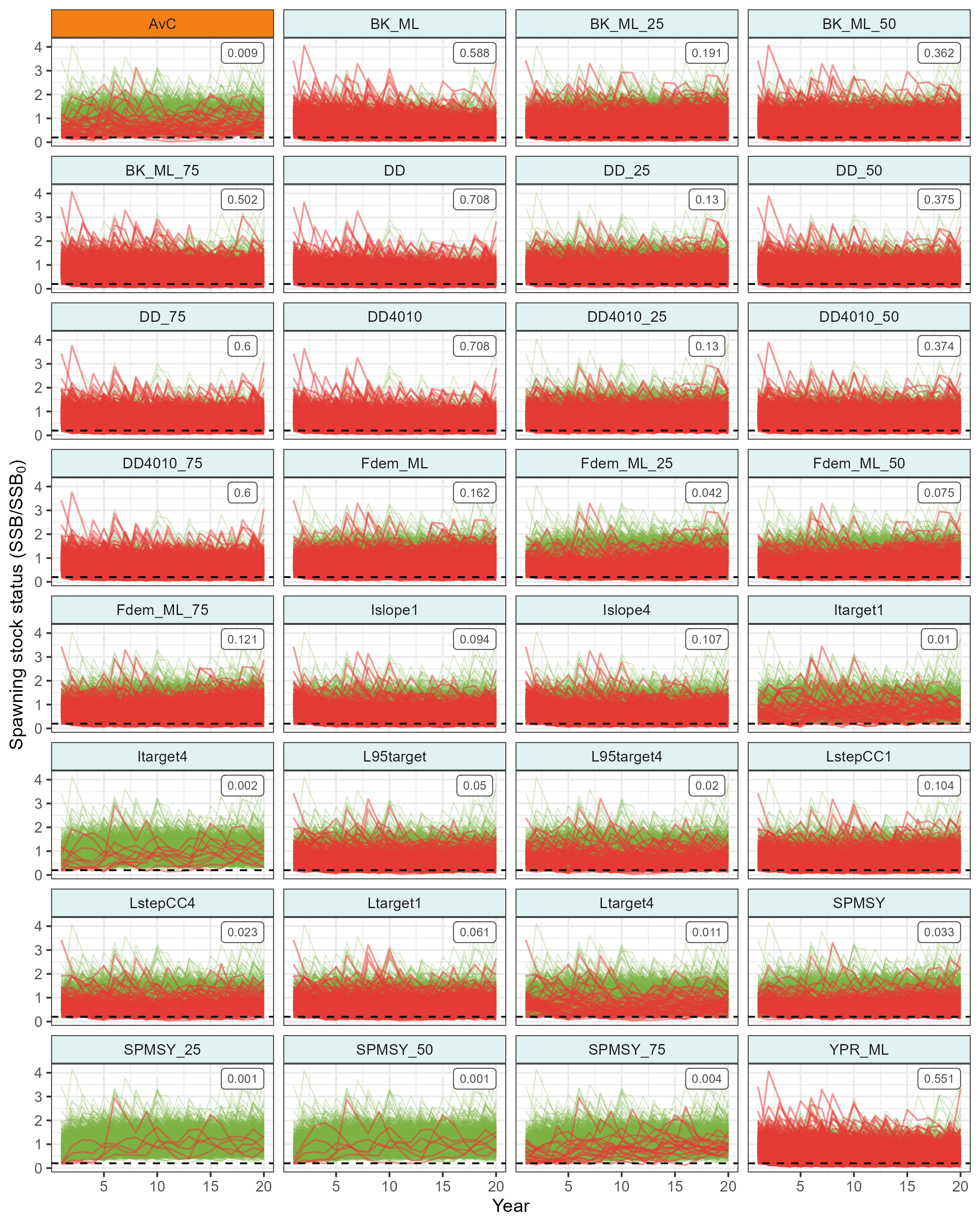
Spawning Stock Status Projections

Code

krill_base_SSS <- reshape2::melt(
  kb_pms$PD@Stat, 
  varnames = c("sim", "mp_idx", "year"), 
  value.name = "SSS") |> 
  dplyr::left_join(MP_idx2name, by = "mp_idx") |> 
  dplyr::mutate(
    below_ref = if_else(min(SSS) < kb_pms$PD@Ref, TRUE, FALSE), 
    .by = c(sim, mp)
  )

krill_base_PD_mtc <- tibble(
  mp = kb_pms$PD@MPs, 
  PD = kb_pms$PD@Mean,
  x = max(krill_base_SSS$year),
  y = max(krill_base_SSS$SSS),
  PF_text = glue("{round(PD, 3)}")
)


p_base_sss <- krill_base_SSS |> 
  ggplot(aes(x = year, y = SSS, group = sim)) +
  geom_path(
    data = ~filter(.x, below_ref == FALSE), 
    alpha = 0.3, 
    color = "#7CB342", 
    linewidth = 0.3
  ) +
  geom_path(
    data = ~filter(.x, below_ref == TRUE), 
    alpha = 0.5, 
    color = "#E53935", 
    linewidth = 0.5
  ) +
  geom_hline(yintercept = kb_pms$PD@Ref, linetype = "dashed") +
  geom_label(
    data = krill_base_PD_mtc,
    #aes(x = x, y = y, label = PF_text),
    aes(x = 18, y = 3.75, label = PF_text),
    #hjust = 1, vjust = 1,
    size = 2.5, colour = "gray25",
    inherit.aes = FALSE
    ) +
  ggh4x::facet_wrap2(.~mp, ncol = 4, strip = MP_strips_theme) +
  labs(
    x = "Year", 
    y = expression(paste("Spawning stock status (SSB/", SSB[0], ")"))
  )

ggsave(
  plot = p_base_sss,
  filename = "outputs/plots/fig_krill_mse_base_SSS_trajectories.png",
  width = 8,
  height = 10
)

Figure 4.1: Simulated trajectories of spawning stock status over time, for Management Procedures under consideration. Dashed line indicates the depletion threshold (0.2). Trajectories that fall below the 0.2 critical depletion threshold are signaled in red. Annotated values denote the PD metric under each MP. The status-quo procedure AvC is highlighted by the orange-shaded panel title background.

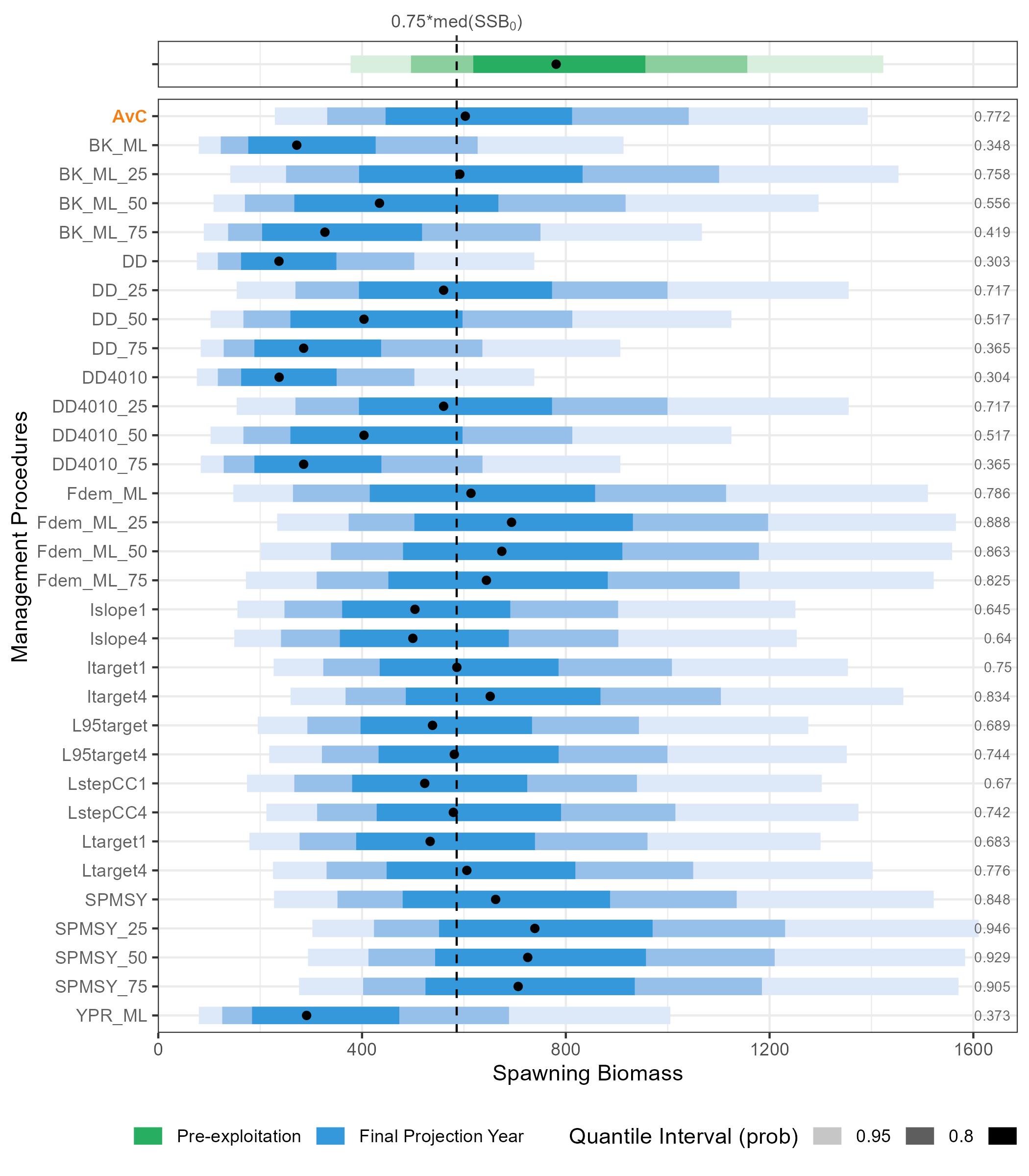
Virgin Spawning Biomass Vs Spawning Biomass in last Projection Year

Code

krill_base_SSBY <- read_rds("outputs/PM_results/krill_base_SSBY.rds") |> 
  reshape2::melt( varnames = c("sim", "mp_idx")) |> 
  dplyr::left_join(MP_idx2name, by = "mp_idx") |> 
  mutate(ssb_type = "Final Projection Year")


krill_base_SSB0 <- tibble(
  value = read_rds("outputs/PM_results/krill_base_SSB0.rds") ,
  sim = 1:length(value),
  mp = "", 
  ssb_type = "Pre-exploitation")


krill_base_ESC_mtc <- tibble(
  mp = kb_pms$ESC@MPs, 
  ESC = kb_pms$ESC@Mean,
  ESC_text = glue("{round(ESC, 3)}"),
  ssb_type = "Final Projection Year") |> 
  mutate(ssb_type = fct_relevel(ssb_type, "Pre-exploitation"))

x_text_col <- ifelse(kb_pms$ESC@MPs == "AvC", col_status_quo, "#616161")
x_text_face <- ifelse(kb_pms$ESC@MPs == "AvC", "bold", "plain")

p_base_ssb0_ssby <- krill_base_SSBY |>
  add_row(krill_base_SSB0) |> 
  mutate(ssb_type = fct_relevel(ssb_type, "Pre-exploitation")) |> 
  ggplot(aes(y = fct_relevel(mp, rev), x = value, color = ssb_type)) +
  ggdist::stat_interval(aes(color_ramp = after_stat(level))) +
  stat_summary(geom = "point", fun = "median", col = "black") +
  geom_vline(aes(xintercept = median(krill_base_SSB0$value)*0.75), linetype = "dashed") +
  geom_text(data = krill_base_ESC_mtc,  aes(x = Inf, y = mp, label = ESC_text), size = 2.5, hjust = 1.2, col = "gray40") +
  labs(x = "Spawning Biomass", y = "Management Procedures") +
  theme(legend.position="bottom") +
  facet_wrap(~ssb_type, strip.position = "right", ncol = 1, scales = "free_y") +
  force_panelsizes(rows = c(0.1, 2)) +
  scale_colour_ramp_discrete(name = "Quantile Interval (prob)")+
  scale_colour_discrete(name = "", type = c("#27AE60", "#3498DB")) +
  guides(
    # emphasize AvC
    y = guide_axis_manual(
      label_colour = rev(x_text_col), 
      label_face = rev(x_text_face)
    ),
    x.sec = guide_axis_manual(
      breaks = median(krill_base_SSB0$value)*0.75,
      labels = expression(paste("0.75*med(", SSB[0], ")")), label_color = "gray30"
      )
  ) +
  theme(
    #remove facet_wrap panels
    strip.background = element_blank(),
    strip.text = element_blank()
  )


ggsave(
  plot = p_base_ssb0_ssby,
  filename = "outputs/plots/fig_krill_mse_base_SSS0_vs_SSBY.png",
  width = 7,
  height = 8
)

Figure 4.2: Quantile intervals (colour-shaded bars) and medians (dots) of simulated pre-explotation spawning biomass (i.e virgin stock, \(SSB_0\), in green) and spawning biomass at the final year of the projection (Year 20, in blue) under each of the considered MPs. Dashed line indicate the critical escapement threshold (i.e. 75% of median \(SSB_0\)). Annotated values denote the ESC metric for each MP. The status-quo procedure AvC is highlighted in orange.

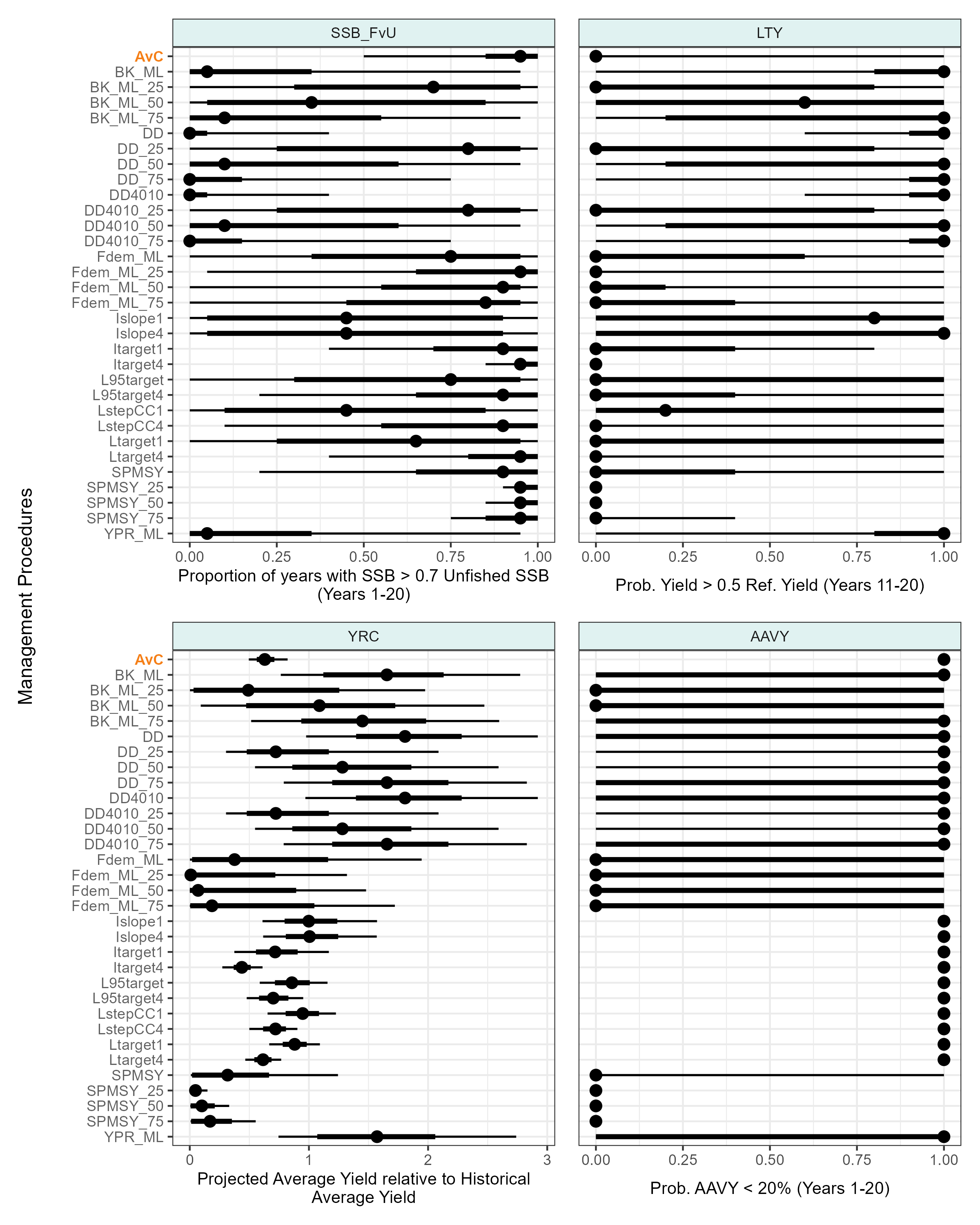
Fished Vs Unfished Spawning Biomass

Code

kb_pms_subset <- kb_pms[c("SSB_FvU", "LTY", "YRC", "AAVY")] |> 
  imap(\(x, y){
    if(y == "YRC"){
      x@Stat |> 
        reshape2::melt( 
          varnames = c("sim", "mp_idx")
        ) |>
        dplyr::left_join(MP_idx2name, by = "mp_idx") |> 
        mutate(
          pm = y, 
          caption = str_wrap(x@Name, 50)
        ) 
    }else{
      x@Prob |> 
        reshape2::melt( 
          varnames = c("sim", "mp_idx")
        ) |>
        dplyr::left_join(MP_idx2name, by = "mp_idx") |> 
        mutate(pm = y, caption = str_wrap(x@Caption, 50))
    }
  })


kb_pms_subset_plots <- kb_pms_subset |> 
  imap(\(x, y){
    
    if(y %in% c("SSB_FvU", "YRC")){
      
      y_text_col <- ifelse(unique(x$mp) == "AvC", col_status_quo, "#616161")
      y_text_face <- ifelse(unique(x$mp) == "AvC", "bold", "plain")
      
      p <- x |> 
        ggplot(aes(y = fct_relevel(mp, rev), x = value)) +
        stat_pointinterval() +
        # stat_interval() +
        # stat_summary(geom = "point", fun = "median", col = "black") +
        # scale_color_brewer() +
        facet_wrap(~pm) +
        labs(x = unique(x$caption), y = "") +
        guides(
          # emphasize AvC
          y = guide_axis_manual(
            label_colour = rev(y_text_col),
            label_face = rev(y_text_face)
          )
        )
    }else{
      p <- x |> 
        ggplot(aes(y = fct_relevel(mp, rev), x = value)) +
        stat_pointinterval() +
        # stat_interval() +
        # stat_summary(geom = "point", fun = "median", col = "black") +
        # scale_color_brewer() +
        facet_wrap(~pm) +
        labs(x = unique(x$caption)) +
        theme(
          axis.title.y = element_blank(),
          axis.text.y = element_blank(),
          axis.ticks.y = element_blank()
        )
    }
    p + theme(axis.title.x = element_text(size = 10))
  })


# Y-axis title-only plot
y_title <- ggplot(data.frame(l = "Management Procedures", x = 1, y = 1)) +
      geom_text(aes(x, y, label = l), angle = 90, size = 4) + 
      theme_void() +
      coord_cartesian(clip = "off")

p_base_pms_sub <- y_title + (wrap_plots(kb_pms_subset_plots, nrow = 2)) + plot_layout(widths = c(1, 25))

ggsave(
  plot = p_base_pms_sub,
  filename = "outputs/plots/fig_krill_mse_base_draws_PMs_subset.png",
  width = 8,
  height = 10
)

Figure 4.3: Point-interval plots for simulated draws of Performance Metrics SSB_FvU, LTY, YRC and AAVY under each considered MP. Dots represent the median, and the thicker and thiner lines represent, respectively, 66% and 95% percentile intervals. The status-quo procedure AvC is highlighted in orange.

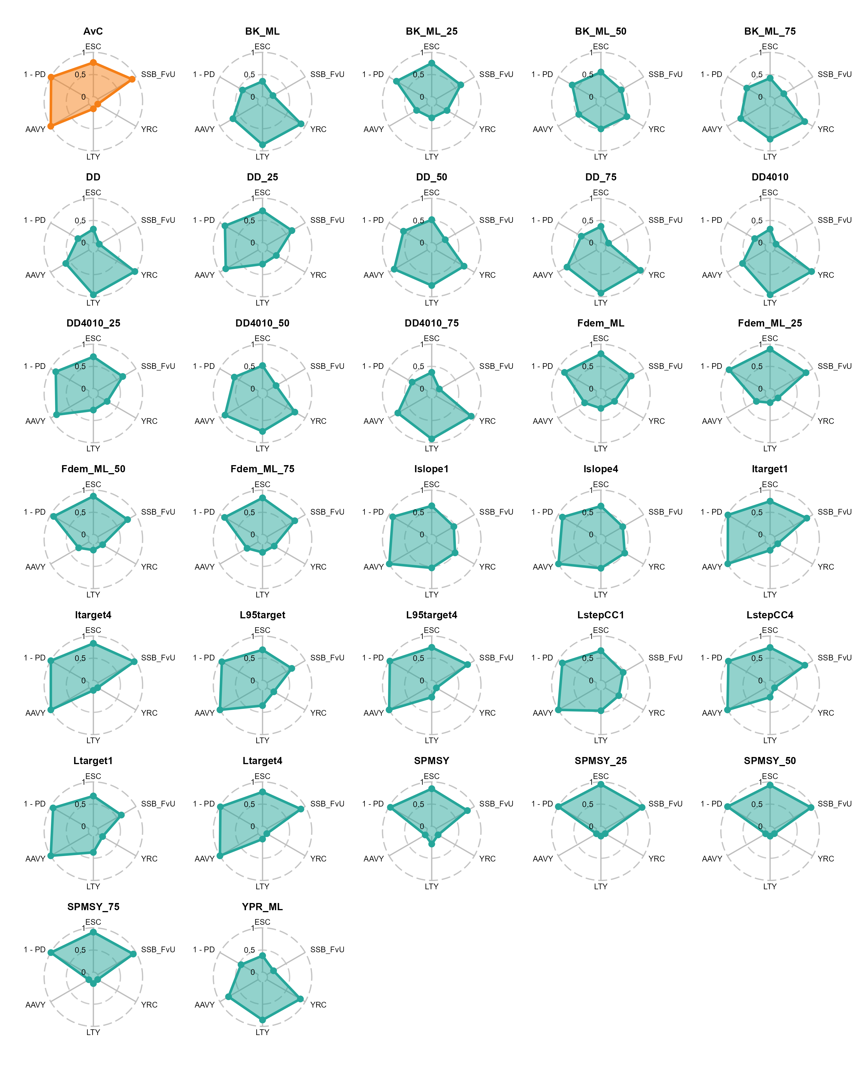
Trade-off plots

Code

radars_base_pms <- kb_pms_summ |> 
  split(f = ~MP) |> 
  map(\(x){
    
    x |> 
      dplyr::select(-PD) |> 
      relocate(`1 - PD`, .after = AAVY) |> 
      ggradar::ggradar(
        values.radar = c(0, 0.5, 1), 
        axis.label.offset = 1.12, 
        # Polygons
        group.line.width = 1, 
        group.point.size = 2,
        group.colours = ifelse(x$MP == "AvC", col_status_quo, "#26A69A"),
        # Background
        background.circle.colour = "white",
        #grid lines
        gridline.label.offset = -.15 * (1 - (0 - ((1/9) * (1 - 0)))),
        gridline.mid.colour = "grey",
        # text size
        axis.label.size = 2.3,
        grid.label.size = 3,
        # general stuff
        fill = TRUE,
        plot.title = x$MP
      ) +
      theme(
        plot.title = element_text(
          size = 8.5, face = "bold", hjust = 0.5, #vjust = -1,
          margin = margin(0, 0, 0, 0)
        ),
        plot.margin = margin(1,1,1,1)
      )
  })

radars_base_pms_export <- wrap_plots(radars_base_pms, ncol = 5)

ggsave(
  plot = radars_base_pms_export,
  filename = "outputs/plots/fig_krill_mse_base_PMs_radars.png",
  width = 10,
  height = 12.5
)

Figure 4.4: Performance Metrics for each of the considered Management Procedures (Table 4.1). All axes are centered at 0, with points further from the centre of the graph indicating better performance (metric PD was reversed to ‘1 - PD’ to comply with that visualization logic). The status-quo procedure AvC is highlighted in orange.

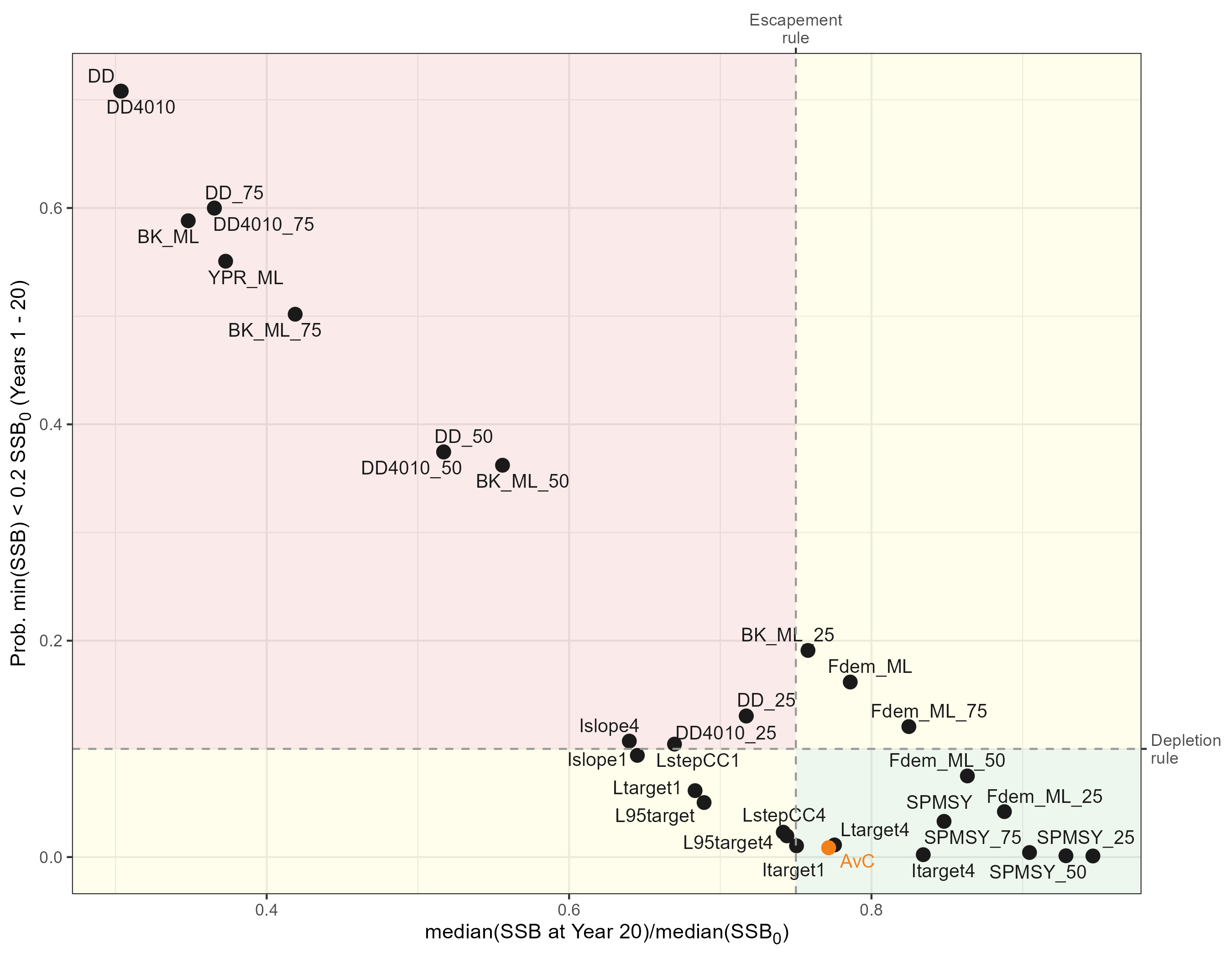
Satisficing CCAMLR’s Precautionary Rules

Code

ccamlr_pd_lim <- 0.1
ccamlr_esc_lim <- 0.75
x_label_pd <- str_replace_all(kb_pms$ESC@Caption, "SSB0", "SSB<sub>0</sub>")
y_label_esc <- str_replace_all(kb_pms$PD@Caption, "SSB0", "SSB<sub>0</sub>")

# Define satisficing areas in plot with associated color shading
# - fail both PD and ESC rules => top-left => red
# - satisfy PD but not ESC => bottom-left => yellow
# - satisfy ESC but not PP => top-right => yellow
# - satisfy both ESC and PP => bottom-right => green
cammlr_areas <- expand_grid(
  position = c("top", "bottom"),
  side = c("left", "right")
) |> 
  mutate(
    area = glue("{position}-{side}"),
    xmin = ifelse(str_detect(area, "left"), -Inf, ccamlr_esc_lim),
    xmax = ifelse(str_detect(area, "left"), ccamlr_esc_lim, Inf),
    ymin = ifelse(str_detect(area, "top"), ccamlr_pd_lim, -Inf),
    ymax = ifelse(str_detect(area, "top"), Inf, ccamlr_pd_lim),
    col = case_when(
      area == "bottom-right" ~ "#4CAF50",
      area == "top-left" ~ "#D32F2F",
      area %in% c("top-right", "bottom-left") ~ "#FFEB3B"
    )
  )

p_satisficing <- kb_pms_summ |> 
  select(MP, PD, ESC) |> 
  mutate(is_status_quo = ifelse(MP == "AvC", "yes", "no")) |> 
  ggplot(aes(x = ESC, y = PD, label = MP, col = is_status_quo)) +
  geom_rect(
    data = cammlr_areas,
    aes(xmin = xmin, xmax = xmax, ymin = ymin, ymax = ymax, fill = col), 
    alpha = 0.1,
    inherit.aes = FALSE
  ) +
  geom_point(size = 3) +
  geom_point(data = ~filter(.x, MP == "AvC"), size = 3) +
  geom_text_repel(size = 3.5) +
  geom_vline(xintercept = ccamlr_esc_lim, linetype = "dashed", col = "gray60") +
  geom_hline(yintercept = ccamlr_pd_lim, linetype = "dashed", col = "gray60") +
  scale_fill_identity() +
  scale_color_manual(values = c("gray10", col_status_quo)) +
  labs(x = x_label_pd, y = y_label_esc) +
  theme(
    axis.title.x = element_markdown(),
    axis.title.y = element_markdown(),
    legend.position = "none"
  ) +
   guides(
     y.sec = guide_axis_manual(
       breaks = 0.1, 
       labels = "Depletion\nrule"),
     x.sec = guide_axis_manual(
       breaks = 0.75, 
       labels = "Escapement\nrule")
   )

ggsave(
  plot = p_satisficing, 
  filename = "outputs/plots/fig_krill_mse_base_ccamlr_satisficing.png",
  width = 9,
  height = 7
)

Figure 4.5: Performance of considered MPs in terms of CCAMLR-based metrics (PD and ESC). Plot split into 3 regions defined based on the satisficing of CCAMLR’s Precautionary rules, i.e. (i) red-shaded area, fails to satisfy the escapement (ESC < 0.75) and depletion (PD < 0.1) rules; (ii) yellow-shaded area, satisfying only one of the rules (yellow); (iii) green-shaded area, satisfying both rules

4.4.1 Robustness Results

Code

# Run PM calculations on each robustness scenario
krill_rbst_pm <- dir_ls(path = "outputs/", regexp = "_rbst_") |> 
  map(\(mse_rbst_path){
    
    mseobj <- read_rds(mse_rbst_path)
    
    list(
      PD = PD(mseobj, Ref = 0.2),
      ESC = ESC(mseobj),
      SSB_FvU = SSB_FvU(mseobj, Ref = 0.70),
      YRC = YRC(mseobj), 
      LTY = LTY(mseobj), 
      AAVY = AAVY(mseobj)
    )
  },  
  .progress = TRUE)

names(krill_rbst_pm) <- str_extract(path_ext_remove(names(krill_rbst_pm)), "(?<=_rbst_)\\w+")

# store outputs
write_rds(krill_rbst_pm, "outputs/PM_results/krill_robustness_PMs_outputs.rds", "gz")

Code

krill_rbst_pm <- read_rds("outputs/PM_results/krill_robustness_PMs_outputs.rds")

# Extract PM summary data 
krill_rbst_pm_sums <- krill_rbst_pm |> 
   # iterate over robustness scenarios
  imap(\(rbst_pms_out, rbst_name){
    rbst_pms_out |>
       # iterate over PM metrics
      imap(\(pm_out, pm_name){ 
        tibble(
          MP = pm_out@MPs, 
          {{pm_name}} := pm_out@Mean
        )
      }) |> 
      reduce(full_join, by = "MP") |> 
      mutate(
        #scn = paste0("rbst_", rbst_name),
        scn = rbst_name, 
        scn_group = "Robustness\nScenarios",
        .before = 1)
  }) |> 
  list_rbind()


# Best MPs based on satisficing both CCAMLR rules (ESC and PD)
base_best_mps <- kb_pms_summ |> 
  select(-`1 - PD`) |> 
  filter(PD < 0.1 & ESC > 0.75) |> 
  mutate(scn = "base", scn_group = "Base\ncase")

Code

# ------------------------------------------------------------------------------
# helper function for tabulating 

# set icons setting trend of robustness scenarios relative to base-case, for each considered MP and  PM
trend_indicator <- function(x, ref){
  case_when(
    x < ref ~ "images/caret-down.png",
    x > ref ~ "images/caret-up.png", 
    .default = "images/minus.png"  
  )
}

satisfy_pd_rule <- function(x){
  ifelse(x > 0.1, "#FFCDD2", "transparent")
}

satisfy_esc_rule <- function(x){
  ifelse(x < 0.75, "#FFCDD2", "transparent")
}
# ---------------------------------------------------------------

# Prepare data for tabulating
krill_rbst_tbl <- krill_rbst_pm_sums |> 
  filter(MP %in% base_best_mps$MP) |> 
  bind_rows(base_best_mps) |> 
  select(-c(scn_group, SSB_FvU:AAVY)) |> 
  pivot_longer(cols = -c(scn, MP), names_to = "PM") |>  
  pivot_wider(names_from = scn, values_from = value) |> 
  relocate(base, .after = PM) |> 
  mutate(across(c(beta:qinc), ~trend_indicator(.x, base), .names = "{.col}_trend"))
  

key_cols <- str_subset(names(krill_rbst_tbl), "trend", negate = TRUE)

krill_rbst_tbl |> 
  flextable(
    col_keys = key_cols
  ) |> 
  add_header_row(
    values = c("Management Procedure", "Performance Metric", "Base Case", "Robustness Scenarios"),
    colwidths = c(1, 1, 1, 5)) |> 
  align(align = "center", part = "all") |>
  set_header_labels(
    MP = "Management Procedure",
    PM = "Performance Metric",
    base = "Base Case",
    beta = "Hyperstability",
    qinc = "Increasing Fishing Efficiency",
    LenCV = "Higher CV in Length-at-age",
    Cbiascv = "Bias in Catch",
    Mbiascv = "Bias in Natural Mortality"
  ) |>  
  merge_v( j = 1:3, part = "header", ) |>
  merge_v(j = ~ MP) |> 
  colformat_double() |> 
  append_chunks(j = ~beta, as_chunk(" "), as_image(src = beta_trend, width = .15, height = .2)) |> 
  append_chunks(j = ~Cbiascv, as_chunk(" "), as_image(src = Cbiascv_trend, width = .15, height = .2)) |> 
  append_chunks(j = ~LenCV, as_chunk(" "), as_image(src = LenCV_trend, width = .15, height = .2)) |> 
  append_chunks(j = ~Mbiascv, as_chunk(" "), as_image(src = Mbiascv_trend, width = .15, height = .2)) |> 
  append_chunks(j = ~qinc, as_chunk(" "), as_image(src = qinc_trend, width = .15, height = .2)) |> 
  highlight(i = ~ PM %in% "PD", j = ~beta + Cbiascv + LenCV + Mbiascv + qinc , color = satisfy_pd_rule) |> 
  highlight(i = ~ PM %in% "ESC", j = ~beta + Cbiascv + LenCV + Mbiascv + qinc, color = satisfy_esc_rule)  |> 
  bg(j = ~ base, bg = "#F5F5F5", part = "all") |> 
  fix_border_issues()

Table 4.4: Comparison of MP performance between the base-case and robustness scenarios, in terms CCAMLR-based metrics PD and ESC. Displayed results restricted to MPs satisfying the CCAMLR’s precautionary rules under the base-case scenario. Symbols denote changes in metric values, i.e. up-arrow for increase, down-arrow for decrease and dash for no change compared to the base-case. Intances where the metric no longer complies with the relevant CCAMLR rule are highlighted in red.

Management Procedure	Performance Metric	Base Case	Robustness Scenarios
			Hyperstability	Bias in Catch	Higher CV in Length-at-age	Bias in Natural Mortality	Increasing Fishing Efficiency
AvC	PD	0.0086	0.0086	0.0088	0.0076	0.0086	0.0086
	ESC	0.7717	0.7717	0.7725	0.7751	0.7717	0.7717
Itarget1	PD	0.0104	0.0098	0.0102	0.0090	0.0104	0.0104
	ESC	0.7504	0.7513	0.7491	0.7538	0.7504	0.7504
Itarget4	PD	0.0022	0.0022	0.0022	0.0020	0.0022	0.0022
	ESC	0.8343	0.8352	0.8354	0.8377	0.8343	0.8343
Ltarget4	PD	0.0112	0.0112	0.0118	0.0102	0.0108	0.0112
	ESC	0.7756	0.7759	0.7779	0.7810	0.7759	0.7756
Fdem_ML_25	PD	0.0420	0.0428	0.0432	0.0578	0.0422	0.0420
	ESC	0.8879	0.8891	0.8900	0.8739	0.8919	0.8879
Fdem_ML_50	PD	0.0750	0.0716	0.0782	0.1170	0.0788	0.0750
	ESC	0.8634	0.8639	0.8626	0.8294	0.8651	0.8634
SPMSY	PD	0.0330	0.0412	0.0378	0.0354	0.0380	0.0330
	ESC	0.8480	0.8454	0.8397	0.8514	0.8363	0.8480
SPMSY_25	PD	0.0010	0.0010	0.0010	0.0008	0.0012	0.0010
	ESC	0.9465	0.9466	0.9442	0.9439	0.9483	0.9465
SPMSY_50	PD	0.0012	0.0016	0.0014	0.0010	0.0010	0.0012
	ESC	0.9286	0.9273	0.9268	0.9288	0.9249	0.9286
SPMSY_75	PD	0.0042	0.0042	0.0040	0.0036	0.0040	0.0042
	ESC	0.9045	0.9025	0.9015	0.9073	0.9031	0.9045

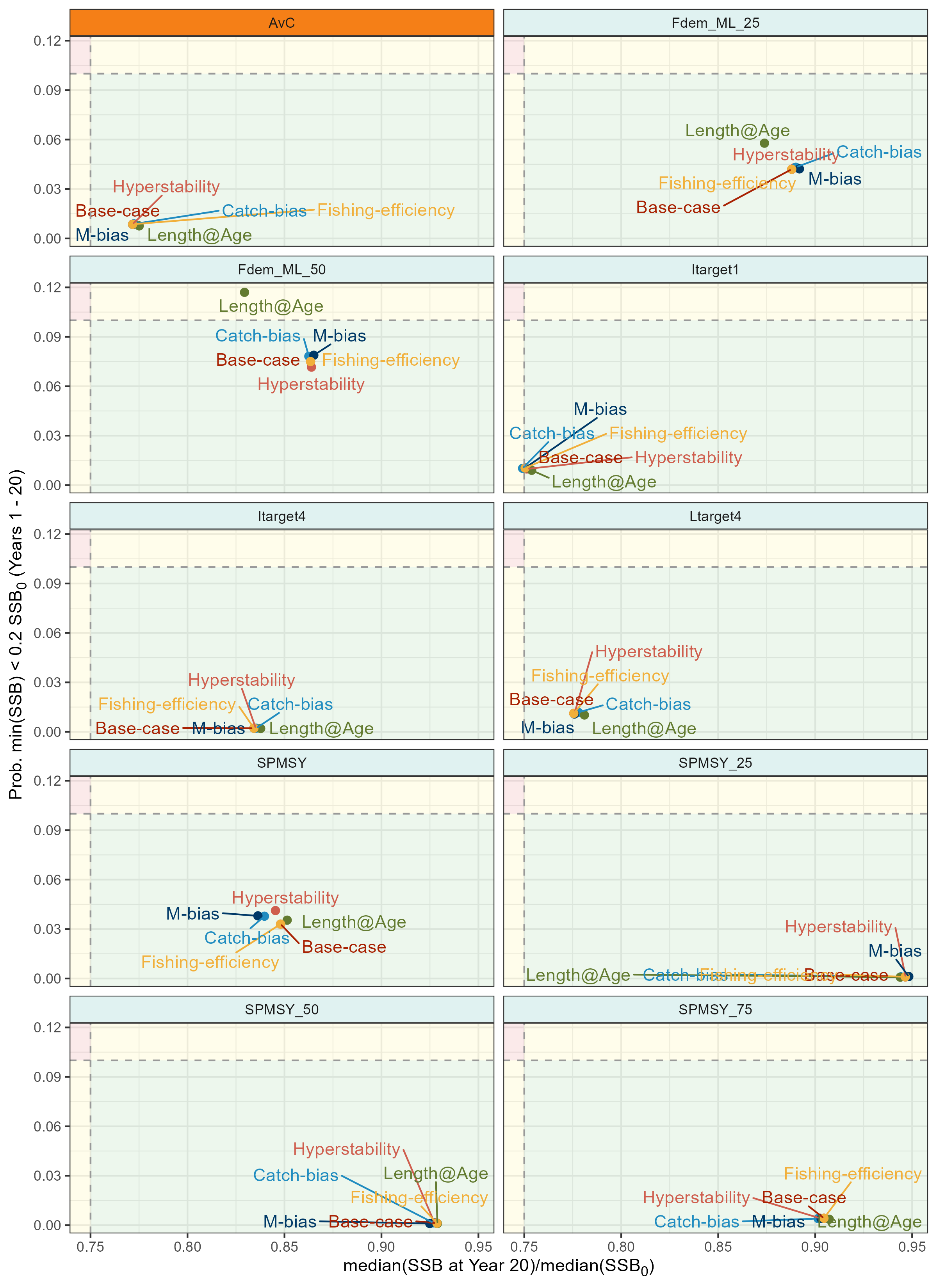
Graphical alternative to above table.

Code

krill_rbst_pm_sums_best <- krill_rbst_pm_sums |>
  filter(MP %in% base_best_mps$MP)

krill_rbst_pm_sums_best <- left_join(krill_rbst_pm_sums_best, rbstn_tbl |> select(c(`Robustness Test ID`, `OM Parameter`)), by = c("scn" = "OM Parameter")) |> 
  select(-scn) |> 
  rename(scn = "Robustness Test ID")


p_robustness <- bind_rows(base_best_mps, krill_rbst_pm_sums_best) |> 
  select(scn, MP, PD, ESC, scn_group) |> 
  mutate(scn = ifelse(scn == "base", "Base-case", scn)) |> 
  ggplot() +
    geom_rect(
    data = cammlr_areas,
    aes(xmin = xmin, xmax = xmax, ymin = ymin, ymax = ymax, fill = col), 
    alpha = 0.1,
    inherit.aes = FALSE
  ) +
  geom_point(aes(x = ESC, y = PD, col = scn), size = 2) +
  geom_text_repel(
    aes(x = ESC, y = PD, col = scn, label = scn), 
    max.overlaps = 15, 
    #fontface = "bold", 
    family = "sans"
  ) +
  geom_vline(xintercept = ccamlr_esc_lim, linetype = "dashed", col = "gray60") +
  geom_hline(yintercept = ccamlr_pd_lim, linetype = "dashed", col = "gray60") + 
  facet_wrap2(vars(MP), ncol = 2, strip = MP_strips_theme) +
  labs(x = x_label_pd, y = y_label_esc) +
  theme(
    axis.title.x = element_markdown(),
    axis.title.y = element_markdown(),
    legend.position = "none"
  ) +
  scale_fill_identity() +
  #scale_color_met_d("Moreau") ++
  scale_color_met_d("Juarez") +
  guides(colour="none")

#p_robustness  

ggsave(
  plot = p_robustness, 
  filename = "outputs/plots/fig_krill_mse_robustness.png",
  width = 8,
  height = 11
)

Figure 4.6: Comparison of performance by Management Procedures (MPs) between the base-case and robustness scenarios (Table 4.3), in terms CCAMLR-based metrics PD and ESC. Displayed results restricted to MPs satisfying the CCAMLR’s precautionary rules under the base-case scenario. Plot split into 3 regions defined based on the satisficing of CCAMLR’s Precautionary rules (similarly to Figure 4.5).

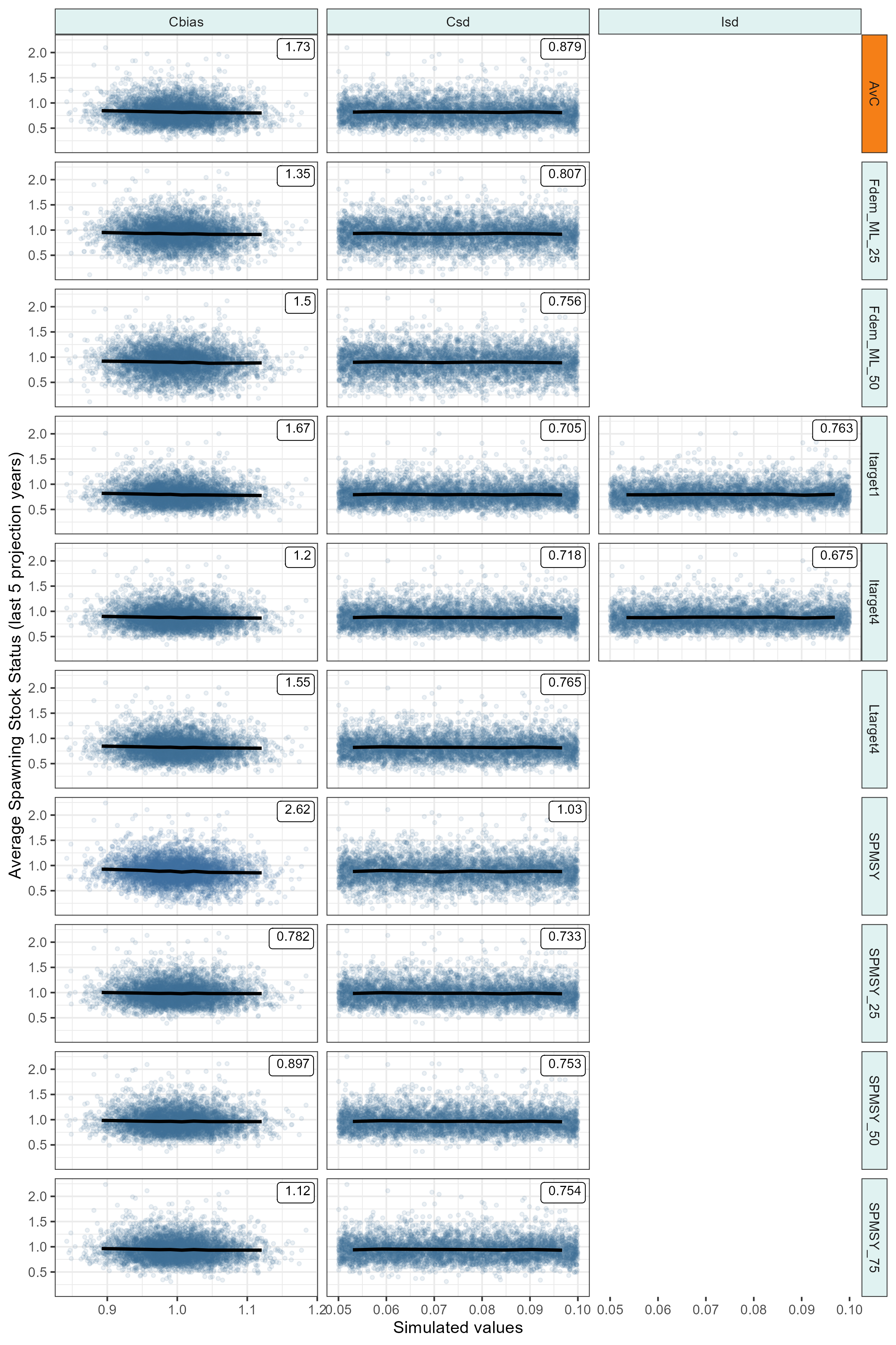
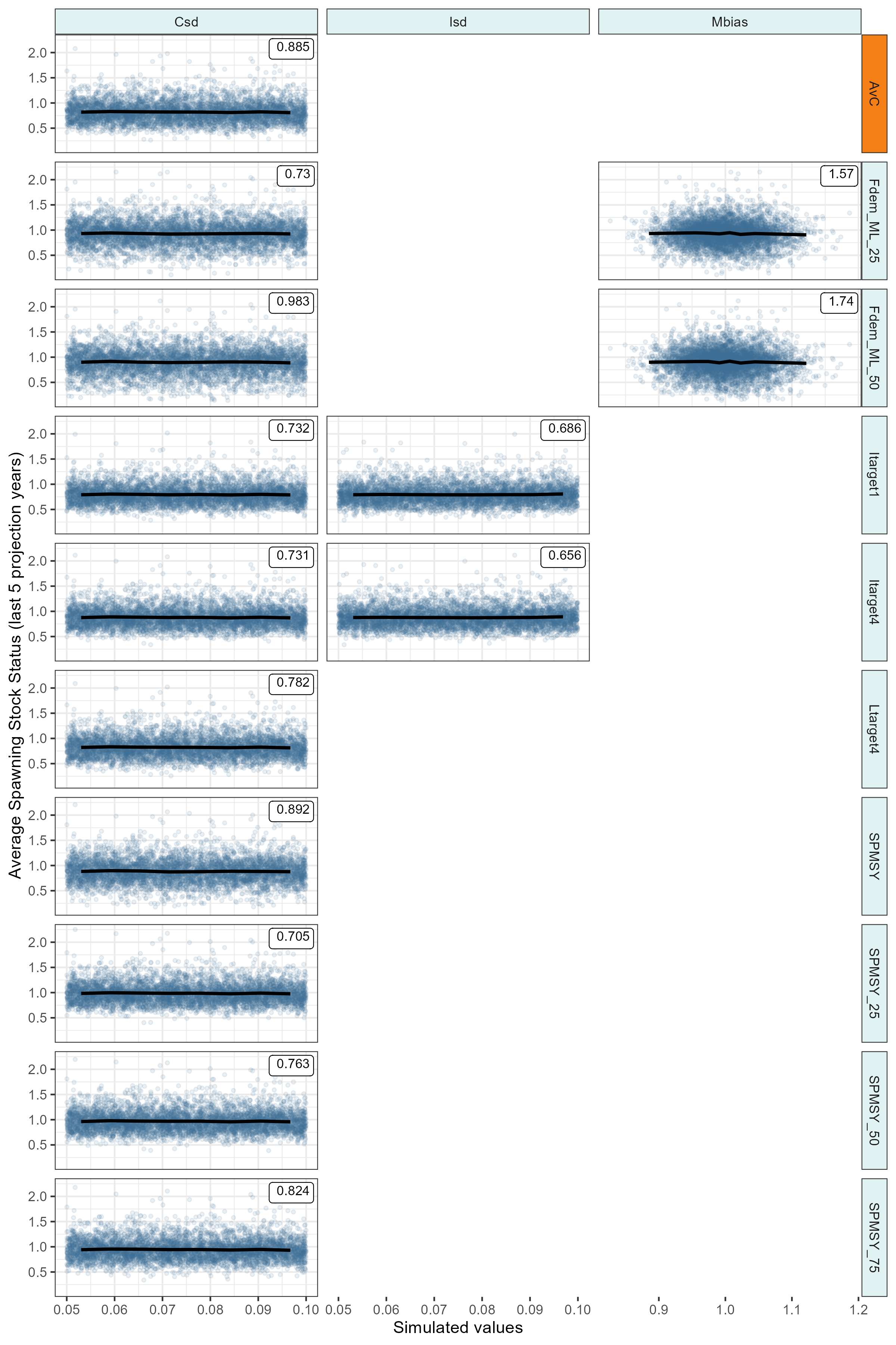
Value of Information plots

Exploring the sensitivity of Management Procedures to variability in the observation process.

Code

source("helpers/VOI_hack.r")

# run VOI calculations for robustness scenarios accounting for observation bias
krill_rbst_voi <- dir_ls(path = "outputs/", regexp = "bias") |> 
  map(\(mse_rbst_path){
    
    mseobj <- read_rds(mse_rbst_path)
    
    mseobj_best <- Sub(mseobj, MPs = base_best_mps$MP)
    
    # calculate average SSS in last 5 years for each simulation (row) and MP (column)
    SSS <- apply(PD(mseobj_best, Yrs = -5)@Stat, c(1, 2), mean)
    
    VOI_hack(
      mseobj_best, 
      Ut = SSS, 
      Utnam = "Average Spawning Stock Status (last 5 projection years)",
      plot = TRUE,
      maxrow = 10, 
      ref_MP = "AvC", col_refMP = col_status_quo, col_otherMP = col_facet_strip_bg
    )
  },  
  .progress = TRUE)

names(krill_rbst_voi) <- str_extract(path_ext_remove(names(krill_rbst_voi)), "(?<=_rbst_)\\w+")

krill_rbst_voi |> 
  iwalk(\(x, y){
    ggsave(
      plot = x$p, 
      filename = paste0("outputs/plots/fig_krill_robustness_voi_", y, ".png"),
      width = 8,
      height = 12
    )
  })

Figure 4.7: Sensitivity of Spawning Stock Status (SSS) to imperfect knowledge in robustness scenario ‘catch-bias’. Panels depict simulated values of SSS (averaged over the last 5 projection years) for a subset of top-performing Management Procedures (one per row) under the base-case scenario. These draws are plotted against those from model parameters describing variability in the observation process (one per column), including bias and error in observed catches (Cbias and Csd) and error in observed indices of abundance (Isd). Displayed panels are determined by data requirements under each MP. Draws of observation variables are grouped into 8 contiguous percentile ranges, and the mean SSS is computed for each range. Black lines connect the means of SSS across the percentile bands, and the annotated values are the CVs (%) of these SSS means, reflecting the marginal effect of observation precision and accuracy on the expected SSS.

Figure 4.8: As for Figure 4.7, but for robusteness scenario ‘M-bias’. The observation variable Mbias describes bias in the estimation of Natural Mortality.

4.5 Session Info

devtools::session_info()

─ Session info ───────────────────────────────────────────────────────────────
 setting  value
 version  R version 4.3.2 (2023-10-31 ucrt)
 os       Windows 11 x64 (build 22621)
 system   x86_64, mingw32
 ui       RTerm
 language (EN)
 collate  English_United Kingdom.utf8
 ctype    English_United Kingdom.utf8
 tz       Europe/London
 date     2023-12-20
 pandoc   3.1.1 @ C:/Program Files/RStudio/resources/app/bin/quarto/bin/tools/ (via rmarkdown)

─ Packages ───────────────────────────────────────────────────────────────────
 !  package           * version  date (UTC) lib source
 P  abind               1.4-5    2016-07-21 [?] CRAN (R 4.3.0)
 P  askpass             1.1      2019-01-13 [?] CRAN (R 4.3.1)
 P  bit                 4.0.5    2022-11-15 [?] CRAN (R 4.3.1)
 P  bit64               4.0.5    2020-08-30 [?] CRAN (R 4.3.1)
 P  bitops              1.0-7    2021-04-24 [?] CRAN (R 4.3.0)
 P  cachem              1.0.8    2023-05-01 [?] CRAN (R 4.3.1)
 P  caTools             1.18.2   2021-03-28 [?] CRAN (R 4.3.1)
 P  cellranger          1.1.0    2016-07-27 [?] CRAN (R 4.3.1)
 P  cli               * 3.6.1    2023-03-23 [?] CRAN (R 4.3.1)
 P  codetools           0.2-19   2023-02-01 [?] CRAN (R 4.3.2)
 P  colorspace          2.1-0    2023-01-23 [?] CRAN (R 4.3.1)
 P  commonmark          1.9.0    2023-03-17 [?] CRAN (R 4.3.1)
 P  crayon              1.5.2    2022-09-29 [?] CRAN (R 4.3.1)
 P  crul                1.4.0    2023-05-17 [?] CRAN (R 4.3.1)
 P  curl                5.0.2    2023-08-14 [?] CRAN (R 4.3.1)
 P  data.table          1.14.8   2023-02-17 [?] CRAN (R 4.3.1)
 P  devtools            2.4.5    2022-10-11 [?] CRAN (R 4.3.2)
 P  digest              0.6.33   2023-07-07 [?] CRAN (R 4.3.1)
 P  distributional      0.3.2    2023-03-22 [?] CRAN (R 4.3.1)
 P  DLMtool           * 6.0.6    2022-06-20 [?] CRAN (R 4.3.1)
 P  dplyr             * 1.1.2    2023-04-20 [?] CRAN (R 4.3.1)
 P  dtplyr            * 1.3.1    2023-03-22 [?] CRAN (R 4.3.1)
 P  ellipsis            0.3.2    2021-04-29 [?] CRAN (R 4.3.1)
 P  equatags            0.2.0    2022-06-13 [?] CRAN (R 4.3.1)
 P  evaluate            0.21     2023-05-05 [?] CRAN (R 4.3.1)
 P  fansi               1.0.4    2023-01-22 [?] CRAN (R 4.3.1)
 P  farver              2.1.1    2022-07-06 [?] CRAN (R 4.3.1)
 P  fastmap             1.1.1    2023-02-24 [?] CRAN (R 4.3.1)
 P  flextable         * 0.9.2    2023-06-18 [?] CRAN (R 4.3.1)
 P  fontBitstreamVera   0.1.1    2017-02-01 [?] CRAN (R 4.3.0)
 P  fontLiberation      0.1.0    2016-10-15 [?] CRAN (R 4.3.0)
 P  fontquiver          0.2.1    2017-02-01 [?] CRAN (R 4.3.1)
 P  forcats           * 1.0.0    2023-01-29 [?] CRAN (R 4.3.1)
 P  fs                * 1.6.3    2023-07-20 [?] CRAN (R 4.3.1)
 P  furrr             * 0.3.1    2022-08-15 [?] CRAN (R 4.3.1)
 P  future            * 1.33.0   2023-07-01 [?] CRAN (R 4.3.1)
 P  gdtools             0.3.3    2023-03-27 [?] CRAN (R 4.3.1)
 P  generics            0.1.3    2022-07-05 [?] CRAN (R 4.3.1)
 P  gfonts              0.2.0    2023-01-08 [?] CRAN (R 4.3.1)
 P  ggblend           * 0.1.0    2023-05-22 [?] CRAN (R 4.3.1)
 P  ggdensity         * 1.0.0    2023-02-09 [?] CRAN (R 4.3.1)
 P  ggdist            * 3.3.0    2023-05-13 [?] CRAN (R 4.3.1)
 P  ggh4x             * 0.2.6    2023-08-30 [?] CRAN (R 4.3.2)
 P  ggplot2           * 3.4.3    2023-08-14 [?] CRAN (R 4.3.1)
    ggradar           * 0.2      2023-12-12 [1] Github (ricardo-bion/ggradar@53404a5)
 P  ggrepel           * 0.9.4    2023-10-13 [?] CRAN (R 4.3.2)
 P  ggtext            * 0.1.2    2022-09-16 [?] CRAN (R 4.3.2)
 P  globals             0.16.2   2022-11-21 [?] CRAN (R 4.3.0)
 P  glue              * 1.6.2    2022-02-24 [?] CRAN (R 4.3.1)
 P  gplots              3.1.3    2022-04-25 [?] CRAN (R 4.3.1)
 P  gridtext            0.1.5    2022-09-16 [?] CRAN (R 4.3.2)
    Grym              * 0.1.1    2023-08-28 [1] Github (AustralianAntarcticDivision/Grym@6a2d6a1)
 P  gtable              0.3.4    2023-08-21 [?] CRAN (R 4.3.1)
 P  gtools              3.9.4    2022-11-27 [?] CRAN (R 4.3.1)
 P  hms                 1.1.3    2023-03-21 [?] CRAN (R 4.3.1)
 P  htmltools           0.5.7    2023-11-03 [?] CRAN (R 4.3.2)
 P  htmlwidgets         1.6.4    2023-12-06 [?] CRAN (R 4.3.2)
 P  httpcode            0.3.0    2020-04-10 [?] CRAN (R 4.3.1)
 P  httpuv              1.6.11   2023-05-11 [?] CRAN (R 4.3.1)
 P  jsonlite            1.8.7    2023-06-29 [?] CRAN (R 4.3.1)
 P  katex               1.4.1    2022-11-28 [?] CRAN (R 4.3.1)
 P  KernSmooth          2.23-22  2023-07-10 [?] CRAN (R 4.3.2)
 P  knitr               1.43     2023-05-25 [?] CRAN (R 4.3.1)
 P  labeling            0.4.2    2020-10-20 [?] CRAN (R 4.3.0)
 P  later               1.3.1    2023-05-02 [?] CRAN (R 4.3.1)
 P  lattice             0.21-9   2023-10-01 [?] CRAN (R 4.3.2)
 P  lifecycle           1.0.3    2022-10-07 [?] CRAN (R 4.3.1)
 P  listenv             0.9.0    2022-12-16 [?] CRAN (R 4.3.1)
 P  lmtest              0.9-40   2022-03-21 [?] CRAN (R 4.3.1)
 P  lubridate         * 1.9.2    2023-02-10 [?] CRAN (R 4.3.1)
 P  magrittr            2.0.3    2022-03-30 [?] CRAN (R 4.3.1)
 P  markdown            1.12     2023-12-06 [?] CRAN (R 4.3.2)
 P  MASS                7.3-60   2023-05-04 [?] CRAN (R 4.3.2)
 P  Matrix              1.6-1.1  2023-09-18 [?] CRAN (R 4.3.2)
 P  memoise             2.0.1    2021-11-26 [?] CRAN (R 4.3.1)
 P  MetBrewer         * 0.2.0    2022-03-21 [?] CRAN (R 4.3.1)
 P  mime                0.12     2021-09-28 [?] CRAN (R 4.3.0)
 P  miniUI              0.1.1.1  2018-05-18 [?] CRAN (R 4.3.2)
 P  MSEtool           * 3.7.0    2023-07-19 [?] CRAN (R 4.3.1)
 P  munsell             0.5.0    2018-06-12 [?] CRAN (R 4.3.1)
 P  mvtnorm           * 1.2-3    2023-08-25 [?] CRAN (R 4.3.1)
 P  nlme                3.1-163  2023-08-09 [?] CRAN (R 4.3.2)
 P  officer             0.6.2    2023-03-28 [?] CRAN (R 4.3.1)
 P  openMSE           * 1.0.0    2021-02-08 [?] CRAN (R 4.3.1)
 P  openssl             2.1.0    2023-07-15 [?] CRAN (R 4.3.1)
 P  openxlsx          * 4.2.5.2  2023-02-06 [?] CRAN (R 4.3.1)
 P  parallelly          1.36.0   2023-05-26 [?] CRAN (R 4.3.0)
 P  patchwork         * 1.1.3    2023-08-14 [?] CRAN (R 4.3.1)
 P  pbapply             1.7-2    2023-06-27 [?] CRAN (R 4.3.1)
 P  pillar              1.9.0    2023-03-22 [?] CRAN (R 4.3.1)
 P  pkgbuild            1.4.3    2023-12-10 [?] CRAN (R 4.3.2)
 P  pkgconfig           2.0.3    2019-09-22 [?] CRAN (R 4.3.1)
 P  pkgload             1.3.3    2023-09-22 [?] CRAN (R 4.3.2)
 P  plyr                1.8.8    2022-11-11 [?] CRAN (R 4.3.1)
 P  profvis             0.3.8    2023-05-02 [?] CRAN (R 4.3.2)
 P  progressr         * 0.14.0   2023-08-10 [?] CRAN (R 4.3.1)
 P  promises            1.2.1    2023-08-10 [?] CRAN (R 4.3.1)
 P  purrr             * 1.0.2    2023-08-10 [?] CRAN (R 4.3.1)
 P  R6                  2.5.1    2021-08-19 [?] CRAN (R 4.3.1)
 P  ragg                1.2.5    2023-01-12 [?] CRAN (R 4.3.1)
 P  Rcpp                1.0.11   2023-07-06 [?] CRAN (R 4.3.1)
 PD RcppParallel        5.1.7    2023-02-27 [?] CRAN (R 4.3.2)
 P  RcppZiggurat        0.1.6    2020-10-20 [?] CRAN (R 4.3.2)
 P  readr             * 2.1.4    2023-02-10 [?] CRAN (R 4.3.1)
 P  readxl            * 1.4.3    2023-07-06 [?] CRAN (R 4.3.1)
 P  remotes             2.4.2.1  2023-07-18 [?] CRAN (R 4.3.1)
    renv                0.17.0   2023-03-02 [1] CRAN (R 4.3.1)
 P  reshape2            1.4.4    2020-04-09 [?] CRAN (R 4.3.1)
 P  Rfast               2.1.0    2023-11-09 [?] CRAN (R 4.3.2)
 P  rlang             * 1.1.1    2023-04-28 [?] CRAN (R 4.3.1)
 P  rmarkdown           2.24     2023-08-14 [?] CRAN (R 4.3.1)
 P  rstudioapi          0.15.0   2023-07-07 [?] CRAN (R 4.3.1)
 P  SAMtool           * 1.6.1    2023-08-23 [?] CRAN (R 4.3.1)
 P  sandwich            3.0-2    2022-06-15 [?] CRAN (R 4.3.1)
 P  scales              1.2.1    2022-08-20 [?] CRAN (R 4.3.1)
 P  sessioninfo         1.2.2    2021-12-06 [?] CRAN (R 4.3.2)
 P  shiny               1.7.5    2023-08-12 [?] CRAN (R 4.3.1)
 P  snow              * 0.4-4    2021-10-27 [?] CRAN (R 4.3.0)
 P  snowfall          * 1.84-6.2 2022-07-05 [?] CRAN (R 4.3.0)
 P  stringi             1.7.12   2023-01-11 [?] CRAN (R 4.3.0)
 P  stringr           * 1.5.0    2022-12-02 [?] CRAN (R 4.3.1)
 P  strucchange         1.5-3    2022-06-15 [?] CRAN (R 4.3.1)
 P  svglite           * 2.1.2    2023-10-11 [?] CRAN (R 4.3.2)
 P  systemfonts         1.0.4    2022-02-11 [?] CRAN (R 4.3.1)
 P  textshaping         0.3.6    2021-10-13 [?] CRAN (R 4.3.1)
 P  tibble            * 3.2.1    2023-03-20 [?] CRAN (R 4.3.1)
 P  tictoc            * 1.2      2023-04-23 [?] CRAN (R 4.3.1)
 P  tidyr             * 1.3.0    2023-01-24 [?] CRAN (R 4.3.1)
 P  tidyselect          1.2.0    2022-10-10 [?] CRAN (R 4.3.1)
 P  tidyverse         * 2.0.0    2023-02-22 [?] CRAN (R 4.3.1)
 P  timechange          0.2.0    2023-01-11 [?] CRAN (R 4.3.1)
 D  TMB                 1.9.6    2023-08-11 [1] CRAN (R 4.3.1)
 P  tzdb                0.4.0    2023-05-12 [?] CRAN (R 4.3.1)
 P  urca                1.3-3    2022-08-29 [?] CRAN (R 4.3.1)
 P  urlchecker          1.0.1    2021-11-30 [?] CRAN (R 4.3.2)
 P  usethis             2.2.2    2023-07-06 [?] CRAN (R 4.3.2)
 P  utf8                1.2.3    2023-01-31 [?] CRAN (R 4.3.1)
 P  uuid                1.1-1    2023-08-17 [?] CRAN (R 4.3.1)
 P  V8                  4.3.3    2023-07-18 [?] CRAN (R 4.3.1)
 P  vars                1.5-9    2023-03-22 [?] CRAN (R 4.3.1)
 P  vctrs               0.6.3    2023-06-14 [?] CRAN (R 4.3.1)
 P  vroom               1.6.3    2023-04-28 [?] CRAN (R 4.3.1)
 P  withr               2.5.0    2022-03-03 [?] CRAN (R 4.3.1)
 P  xfun                0.40     2023-08-09 [?] CRAN (R 4.3.1)
 P  xml2                1.3.5    2023-07-06 [?] CRAN (R 4.3.1)
 P  xslt                1.4.4    2023-02-21 [?] CRAN (R 4.3.1)
 P  xtable              1.8-4    2019-04-21 [?] CRAN (R 4.3.1)
 P  yaml                2.3.7    2023-01-23 [?] CRAN (R 4.3.0)
 P  zip                 2.3.0    2023-04-17 [?] CRAN (R 4.3.1)
 P  zoo                 1.8-12   2023-04-13 [?] CRAN (R 4.3.1)

 [1] C:/Users/bruno/Dropbox/krill/krill_mse/renv/library/R-4.3/x86_64-w64-mingw32
 [2] C:/Users/bruno/AppData/Local/R/cache/R/renv/sandbox/R-4.3/x86_64-w64-mingw32/7df9739c

 P ── Loaded and on-disk path mismatch.
 D ── DLL MD5 mismatch, broken installation.

──────────────────────────────────────────────────────────────────────────────

#library(gratitude)

CCAMLR Secretariat. 2023. “CCAMLR Statistical Bulletin, Vol. 35.” https://www.ccamlr.org/en/document/data/ccamlr-statistical-bulletin-vol-35.

Constable, A, and W. de la Mare. 1996. “A Generalised Model for Evaluating Yield and the Long-Term Status of Fish Stocks Under Conditions of Uncertainty.” CCAMLR Science 3: 31–54.

Kawaguchi, So. 2016. “Reproduction and Larval Development in Antarctic Krill (Euphausia Superba).” In Biology and Ecology of Antarctic Krill, edited by Volker Siegel, 225–46. Advances in Polar Ecology. Cham: Springer International Publishing. https://doi.org/10.1007/978-3-319-29279-3_6.

Maschette, D, S Wotherspoon, S Kawaguchi, and Philippe Ziegler. 2021. “Grym Assessment for Subarea 48.1 Euphausia Superba Populations.” WG-FSA-2021/39. Hobart, Autralia: CCAMLR. https://meetings.ccamlr.org/en/wg-fsa-2021/39.

Pakhomov, E. A. 1995. “Natural Age-Dependent Mortality Rates of Antarctic Krill Euphausia Superba Dana in the Indian Sector of the Southern Ocean.” Polar Biology 15 (1): 69–71. https://doi.org/10.1007/BF00236127.

SC-CAMLR. 2000. “Report of the Bo Workshop.” SC-CAMLR-XIX. Annex 4, Appendix G. CCAMLR.

Thanassekos, S, K Reid, S Kawaguchi, S Wotherspoon, D Maschette, P Ziegler, D Welsford, et al. 2021. “Grym Parameter Values for Subareas 48.1, 48.2 and 48.3.” WG-SAM-2021/12. CCAMLR.